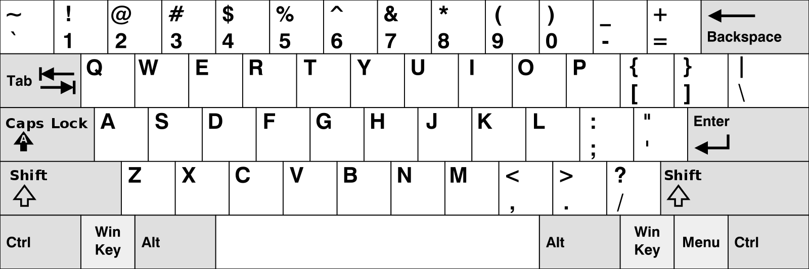
中国大陆键盘布局（keyboard layout）和美国一样，即美式键盘（QWERTY）。

Chinese keyboard layout QWERTY [1]

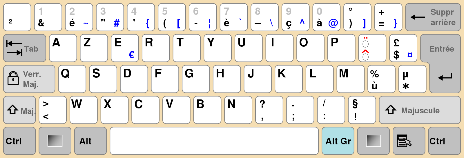
French keyboard layout AZERTY [1]

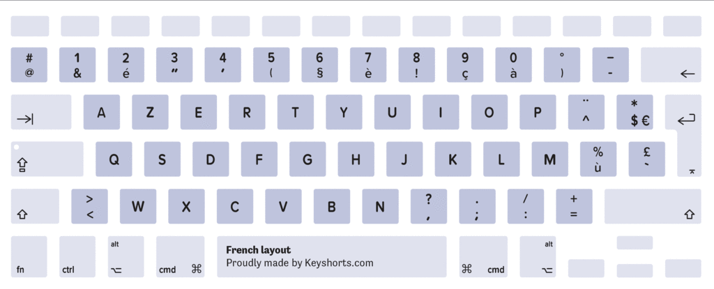
French keyboard layout AZERTY (MacBook or Apple keyboard) [2]

References

[1] 键盘布局. (2009, June 7). 维基百科，自由的百科全书. https://zh.wikipedia.org/wiki/%E9%94%AE%E7%9B%98%E5%B8%83%E5%B1%80

[2] Keyshorts. (2015, July 17). How to identify MacBook keyboard layout? https://keyshorts.com/blogs/blog/37615873-how-to-identify-macbook-keyboard-localization#french

Let’s say we have input data $X$ and we want to classify the data into labels $Y$.

• A generative model (生成模型) learns the joint probability distribution $\mathbb{P}(X, Y)$
• A discriminative model (判别模型) learns the conditional probability distribution $\mathbb{P}(Y | X)$

Discriminative models learn the (hard or soft) boundary between classes, generative models model the distribution of individual classes.

Examples of generative models:

• HMM (hidden markov model)
• Naive Bayes
• Gaussian mixture model and other types of mixture model
• GAN (generative adversarial network)
• VAE (variational autoencoder)
• PCFG (probabilistic context-free grammar)
• Latent Dirichlet allocation
• Boltzmann machine

Examples of discriminative models:

• CRF (conditional random field)
• Logistic regression
• SVM
• Decision tree
• Random forest
• KNN (k-nearest neighbors)
• Neural networks
• Classical (sparse, denoising, etc.) autoencoders are generally classified as discriminative models, although denoising autoencoders can be used as generative models [1].

For sequence labeling tasks (such as Part-of-Speech tagging and Name Entity Recognition), discriminative models are said to be preferred to generative models [2].

There is a widely-held belief that discriminative models are almost always to be preferred in classification tasks [3].

One of the advantages of generative models is that they can be used to generate new data similar to existing data.

References

[1] Bengio, Y., Yao, L., & Alain, P. (2013). Generalized Denoising Auto-Encoders as Generative ModelsarXiv e-prints, arXiv:1305.6663.

[2] Why discriminative models are preferred to generative models for sequence labeling tasks? (n.d.). Cross Validated. https://stats.stackexchange.com/questions/73015/why-discriminative-models-are-preferred-to-generative-models-for-sequence-labeli

[3] Andrew Y. Ng and Michael I. Jordan, On discriminative vs. generative classifiers: A comparison of logistic regression and naive bayes, Advances in Neural Information Processing Systems 14 (T. G. Dietterich, S. Becker, and Z. Ghahramani, eds.), MIT Press, 2002, pp. 841–848.

• true positive (TP)
• true negative (TN)
• false positive (FP)
  • type I error: rejection of a true null hypothesis
• false negative (FN)
  • type II error: non-rejection of a false null hypothesis

Confusion matrix:

Accuracy can be a misleading metric for imbalanced data sets because it can be biased by the most common target class.

A high sensitivity test is reliable when its result is negative since it rarely misdiagnoses the cases which are indeed positive, it is not that reliable when its result is positive.

A high specificity test is reliable when its result is positive since it rarely gives positive results in negative cases, it is not that reliable when its result is negative. A test with a higher specificity has a lower type I error rate.

The ROC curve is created by plotting the true positive rate (TPR) against the false positive rate (FPR) at various threshold settings. True positive rate (TPR) is also known as recall, sensitivity or probability of detection. false positive rate (FPR) can be calculated as $1 - \text{specificity}$.

The precision-recall curve (PR curve) shows the tradeoff between precision and recall for different threshold.

According to a post on Cross-Validated, the key difference is that ROC curves will be the same no matter what the baseline probability is, but PR curves may be more useful in practice for problems where the positive class is more interesting than the negative class (imbalanced problems). Recall (sensitivity) and specificity, which make up the ROC curve, are probabilities conditioned on the true class label. Precision is a probability conditioned on the estimate of the class label. If the question is: “How meaningful is a positive result from the classifier given the baseline probabilities of the problem?”, use a PR curve. If the question is, “How well can this classifier be expected to perform in general, at a variety of different baseline probabilities?”, go with a ROC curve.

The general definition for the Average Precision (AP) is finding the area under the precision-recall curve. Before calculating AP for the object detection, we often smooth out the zig-zag pattern first. Graphically, at each recall level, we replace each precision value with the maximum precision value to the right of that recall level.

mAP (mean average precision) is the average of AP. In some context, we compute the AP for each class and average them to get mAP. But in some context, for example, under the COCO context, AP is averaged over all classes (even also over several IoU thresholds), which is traditionally called mAP.

How is precision-recall curve drawn?

• In the context of object detection, we first rank the predicted bounding boxes by their corresponding confidence score. By following this ranking, we cumulatively (only considering the current bounding box and all previous bounding boxes) calculate pairs of precision and recall. For each precision-recall pair, we draw a point in the precision-recall curve. By following this ranking, the recall of successive pairs will be increasing (not strictly increasing) by nature, on the other hand the precision can have a zig-zag pattern because of newly encountered false-positive predicted bounding boxes. This is why precision-recall curve is usually smoothed.

Comparison of F1 score and AP:

• F1 score is sensitive to the trade-off between precision and recall. Therefore, careful tuning is often needed to get the best combination of precision and recall. On the other hand, AP is invariant to that trade-off. AP, on the other hand, calculates a measure by iterating over all points of precisions and recalls. Thus, it is invariant to the trade-off between precision and recall.
• For each point of the precision-recall curve (each pair of precision+recall), one can obtain a F1 score. One can then choose to keep the maximum one among obtained F1 scores.

Correlation

To compute the correlation between two time series, we can use the .corr() method of pandas.Series.

To visualize the scatter plot of two time series:

1
2
3
4
5
6
7
8
9
10
11
12
13
14
15
16
17
18

def correlation_between_2_ts(s1, s2, figsize=(5, 5), plot_scatter=True):
    """
    Computes correlation between two time series
    
    s1, s2: named pandas.Series 
    """
    correlation = s1.corr(s2)
    if plot_scatter:
        plt.figure(figsize=figsize)
        plt.scatter(s1, s2)
        plt.grid()
        title = "Scatter plot of {} and {}".format(s1.name, s2.name) 
        title += "\ncorrelation = {:.4f}".format(correlation)
        plt.title(title) 
        plt.show()
    return correlation

correlation = correlation_between_2_ts(s1, s2)

Autocorrelation function (ACF)

The autocorrelation as a function of the lag. It equals one at lag-zero.

1
2
3

from statsmodels.tsa.stattools import acf

acf(data)

1
2
3
4

from statsmodels.graphics.tsaplots import plot_acf

plot_acf(data, alpha=0.05, lags=30)
plt.show()

To compute a single lag-N autocorrelation, we can also use the .autocorr(lag=N) method of pandas.Series.

Stationarity

• Strong stationarity: joint distribution of the observations is time-invariant.
• Weak stationarity: mean, variance and autocorrelation of the observations are time-invariant. For autocorrelation, $\text{corr}(X_t, X_{t-\tau})$ is only a function of $\tau$, not $t$.
• Weak stationarity is easier to test than strong stationarity.
• If a process is not stationary, it becomes difficult to model. Modeling involves estimating a set of parameters. If a process is not stationary and the parameters are different at each point in time, then there are too many parameters to estimate (maybe more parameters than data).
• A random walk is a common type of non-stationary series, its variance grows with time. Seasonal series are also non-stationary, for example, its mean varies with time. A white noise series with varying mean is non-stationary.
• A white noise series (with constant mean and variance) is stationary.
• Many non-stationary series can be made stationary through a simple transformation. For example, if we take the differences (with a lag of $1$) of a random walk series, we get a white noise series. A seasonal series can be made stationary by seasonal adjustments (taking the difference with a lag corresponding to the periodicity). Most economic data published by the government is seasonally adjusted. Sometimes, we may need more than one transformations, for a series that grows exponentially and shows a strong seasonal pattern, we can first take the log of the series to eliminate the exponential growth and then a seasonal difference. These operations often involve df.diff(), np.log(), np.sqrt(), etc.

White noise

White noise is a series with:

• constant mean
• constant variance
• zero autocorrelations at all lags
• special case: if data has normal distribution, then Gaussian white noise

1

gaussian_white_noise = np.random.normal(loc=0.02, scale=0.05, size=1000)

Random walk

In other words, the change is white noise:

One cannot forecast a random walk, the best forecast for the next value is the current value.

An extension, random walk with drift:

Augmented Dickey-Fuller test

The Dickey-Fuller test is the following:

Null hypothesis: $H_0 : \phi = 1$

This is equivalent to:

Null hypothesis: $H_0 : \phi = 0$

If we add more lagged changes on the right hand side, it’s the Augmented Dickey-Fuller test.

The null hypothesis for both Dickey-Fuller test and Augmented Dickey-Fuller test is that the data are non-stationary.

If we use $5\%$ as the threshold, a p-value less than $5\%$ indicates that:

• we can reject the null hypothesis that the series is non-stationary with $95\%$ confidence.
• this series is stationary.

If we use $5\%$ as the threshold, a p-value larger than $5\%$ indicates that:

• we cannot reject the null hypothesis.
• this series is non-stationary.

1
2
3
4

from statsmodels.tsa.stattools import adfuller

# p-value
adfuller(p1)[1]

Autoregressive model (AR model)

AR model of order $1$, or simply AR$(1)$ model (there is only one lagged value on right hand side):

If AR parameter $\phi = 1$, then this is a random walk. If $\phi = 0$, then this is white noise.

In order for the process to be stable and stationary, $\phi$ has to be $- 1 < \phi < 1$.

Interpretation of AR$(1)$ parameter:

• negative $\phi$: mean reversion
• positive $\phi$: momentum.
• the autocorrelation function decays exponentially for an AR$(1)$ time series at a rate of the AR$(1)$ parameter $\phi$.

The model can be extended to include more lagged values and more $\phi$ parameters:

• AR$(1)$: $X_t = \mu + \phi_1 X_{t-1} + \epsilon_t$
• AR$(2)$: $X_t = \mu + \phi_1 X_{t-1} + \phi_2 X_{t-2} + \epsilon_t$
• etc.

To simulate AR time series, take care of the convention: we must include the zero-lag coefficient of $1$ and the sign of the other coefficients is opposite what we have been using above.

1
2
3
4
5
6
7
8
9
10
11
12
13

from statsmodels.tsa.arima_process import ArmaProcess

# phi = + 0.9
ar = [1, - 0.9]
ma = [1]
arma_process = ArmaProcess(ar, ma)
simulated_data = arma_process.generate_sample(nsample=1000)

# phi = - 0.9
ar = [1, 0.9]
ma = [1]
arma_process = ArmaProcess(ar, ma)
simulated_data = arma_process.generate_sample(nsample=1000)

To estimate an AR model (estimate parameters from data):

1
2
3
4
5
6
7

from statsmodels.tsa.arima_model import ARMA

# Fit an AR(1) model to the data, true phi = + 0.9
arma = ARMA(data, order=(1, 0))
arma_results = arma.fit()

print(arma_results.summary())

1
2
3
4
5
6
7
8
9
10
11
12
13
14
15
16
17
18
19
20
21

                              ARMA Model Results                              
==============================================================================
Dep. Variable:                      y   No. Observations:                 1000
Model:                     ARMA(1, 0)   Log Likelihood               -1455.318
Method:                       css-mle   S.D. of innovations              1.036
Date:                Sun, 12 Apr 2020   AIC                           2916.636
Time:                        20:45:48   BIC                           2931.360
Sample:                             0   HQIC                          2922.232
                                                                              
==============================================================================
                 coef    std err          z      P>|z|      [0.025      0.975]
------------------------------------------------------------------------------
const         -0.0938      0.323     -0.290      0.772      -0.727       0.540
ar.L1.y        0.8995      0.014     65.170      0.000       0.872       0.927
                                    Roots                                    
=============================================================================
                  Real          Imaginary           Modulus         Frequency
-----------------------------------------------------------------------------
AR.1            1.1117           +0.0000j            1.1117            0.0000
-----------------------------------------------------------------------------

We can do forecasting, both in-sample and out-of-sample using statsmodels. The in-sample is a forecast of the next data point using the data up to that point, and the out-of-sample forecasts any number of data points in the future. These forecasts can be made using either the predict() method if we want the forecasts in the form of a series of data, or using the plot_predict() method if we want a plot of the forecasted data. We supply the starting point for forecasting and the ending point, which can be any number of data points after the data set ends. plot_predict() also gives confidence intervals around the out-of-sample forecasts.

1
2
3

1
2
3

# Plot the original series and the forecasted series
arma_results.plot_predict(start=0, end="2030")
plt.show()

To identify the order of an AR model:

• Partial autocorrelation function (PACF) meansures the incremental benefit of adding another lag. Each coefficient of PACF represents how significant adding the corresponding lag when we already have all the previous lags included.
• Information criteria computes the goodness-of-fit with the estimated parameters, but apply a penalty function on the number of parameters in the model. In general, the more parameters in a model, the better the model will fit the data. But this can lead to overfitting. There are two popular information criteria:
  • AIC (Akaike Information Criterion)
  • BIC (Bayesian Information Criterion)

In practice, the way to use the information criteria is to fit several models, each with a different number of parameters, and choose the one with the lowest information criteria. Compared to AIC, BIC penalizes additional model orders more than AIC and so the BIC will sometimes suggest a simpler model. The AIC and BIC will often choose the same model, but when they don’t we have to make a choice. If our goal is to identify good predictive models, we should use AIC. If our goal is to identify a good explanatory model, we should use BIC.

1
2
3
4

from statsmodels.graphics.tsaplots import plot_pacf

plot_pacf(data, lags=20)
plt.show()

1
2
3
4
5
6
7
8
9
10
11
12
13

from statsmodels.tsa.arima_model import ARMA

bic = []
range_ = range(1, 7)
for p in range_:
    arma = ARMA(simulated_data, order=(p, 0))
    arma_results = arma.fit()  
    bic.append(arma_results.bic)

plt.plot(range_, bic, marker="o")
plt.xlabel("Order of AR Model")
plt.ylabel("BIC")
plt.show()

Moving average model (MA model)

MA model of order $1$, or simply MA$(1)$ model (there is only one lagged error on right hand side):

If MA parameter $\theta = 0$, then this is white noise.

MA models are stationary for all values of $\theta$.

Interpretation of MA$(1)$ parameter:

• negative $\theta$: one-period mean reversion
• positive $\theta$: one-period momentum
• one-period autocorrelation (lag-$1$ autocorrelation) is not $\theta$, it is $\frac{\theta}{1 + \theta^2}$. There is zero autocorrelation for an MA$(1)$ beyond lag-$1$.
• higher frequency stock data is well modeled by an MA$(1)$ process. For example, one day’s prices (on September 1, 2017) for Sprint stock (ticker symbol “S”) sampled at a frequency of one minute. The stock market is open for 6.5 hours (390 minutes), from 9:30am to 4:00pm. Such data can be accessed via Google Finance [3]. Stocks trade at discrete one-cent increments (although a small percentage of trades occur in between the one-cent increments) rather than at continuous prices, and when we plot the data we should observe that there are long periods when the stock bounces back and forth over a one cent range. This is sometimes referred to as “bid/ask bounce”. The bouncing of the stock price between bid and ask induces a negative first order autocorrelation, but no autocorrelations at lags higher than $1$.

The model can be extended to include more lagged errors and more $\theta$ parameters:

• MA$(1)$: $X_t = \mu + \epsilon_t + \theta_1 \epsilon_{t-1}$
• MA$(2)$: $X_t = \mu + \epsilon_t + \theta_1 \epsilon_{t-1} + \theta_2 \epsilon_{t-2}$
• etc.

An MA$(q)$ model has no autocorrelation beyond lag-$q$.

To simulate MA time series, take care of the convention: we must include the zero-lag coefficient of $1$. However, unlike with the AR simulation, we don’t need to reverse the sign of $\theta$, its sign is what we have been using above.

1
2
3
4
5
6
7
8
9
10
11
12
13

from statsmodels.tsa.arima_process import ArmaProcess

# theta = + 0.9
ar = [1]
ma = [1, 0.9]
arma_process = ArmaProcess(ar, ma)
simulated_data = arma_process.generate_sample(nsample=1000)

# theta = - 0.9
ar = [1]
ma = [1, - 0.9]
arma_process = ArmaProcess(ar, ma)
simulated_data = arma_process.generate_sample(nsample=1000)

To estimate an MA model (estimate parameters from data):

1
2
3
4
5
6
7

from statsmodels.tsa.arima_model import ARMA

# Fit an MA(1) model to the data, true theta = + 0.9
arma = ARMA(data, order=(0, 1))
arma_results = arma.fit()

print(arma_results.summary())

1
2
3
4
5
6
7
8
9
10
11
12
13
14
15
16
17
18
19
20

                              ARMA Model Results                              
==============================================================================
Dep. Variable:                      y   No. Observations:                 1000
Model:                     ARMA(0, 1)   Log Likelihood               -1404.378
Method:                       css-mle   S.D. of innovations              0.985
Date:                Mon, 13 Apr 2020   AIC                           2814.756
Time:                        16:10:50   BIC                           2829.479
Sample:                             0   HQIC                          2820.352
                                                                              
==============================================================================
                 coef    std err          z      P>|z|      [0.025      0.975]
------------------------------------------------------------------------------
const         -0.0664      0.060     -1.112      0.266      -0.184       0.051
ma.L1.y        0.9203      0.012     75.882      0.000       0.896       0.944
                                    Roots                                    
=============================================================================
                  Real          Imaginary           Modulus         Frequency
-----------------------------------------------------------------------------
MA.1           -1.0867           +0.0000j            1.0867            0.5000
-----------------------------------------------------------------------------

Just as with AR models, we can use MA models to do forecasting, both in-sample and out-of-sample using statsmodels. This can be done via either the predict() method if we want the forecasts in the form of a series of data, or the plot_predict() method if we want a plot of the forecasted data. One big difference between out-of-sample forecasts with an MA$(1)$ model and an AR$(1)$ model is that the MA$(1)$ forecasts more than one period in the future are simply the mean of the sample.

1
2
3

1
2
3

# Plot the original series and the forecasted series
arma_results.plot_predict(start=0, end="2030")
plt.show()

Autoregressive moving average model (ARMA model)

An ARMA model is a combination of an AR model and an MA model.

ARMA$(1, 1)$ model:

ARMA models are generally denoted ARMA$(p, q)$ where parameters $p$ and $q$ are non-negative integers, $p$ is the order of the AR model, $q$ is the order of the MA model.

ARMA models can be converted to pure AR or pure MA models. Here is an example of converting an AR$(1)$ model into an an MA$(\infty)$:

This demonstrates that an AR$(1)$ model is equivalent to an MA$(\infty)$ model with the appropriate parameters.

Using ACF and PACF to choose model order

The time series must be made stationary before making these plots. If the ACF values are high and tail off very very slowly, this is the sign that the data is non-stationary, so it needs to be differenced. If the autocorrelation at lag-$1$ is very negative, this is the sign that we have taken the difference too many times.

In the case of ARMA$(p, q)$, we cannot deduce the model orders $p$ and $q$ from the plots. However, we can use AIC and BIC to find the most appropriate $p$ and $q$. Sometimes when searching over model orders we will attempt to fit an order that leads to an error, for example, ValueError: Non-stationary starting augoregressive parameters found with enforce_stationary set to True. This ValueError tells us that we have tried to fit a model which would result in a non-stationary set of AR coefficients. We can use try/except blocks to skip this one.

Cointegration model

The idea behind cointegration (协整) is that even if the prices of two different assets both follow random walks, it is still possible that a linear combination of them is not a random walk. If that’s true, then even though these two assets are not forecastable because they are random walks, the linear combination is forecastable. We say that these two assets are cointegrated. One analogy is that a dog owner walking his dog with a retractable leash. The position of the dog owner and the position of the dog may both follow random walks, but the distance between them may very well be mean reverting. Examples can be found by looking at economic substitutes: heating oil and natural gas, platinum and palladium, corn and wheat, corn and sugar, Bitcoin and Ethereum, etc. For stocks, a natural starting point for identifying cointegrated pairs are stocks in the same industry. However competitors are not necessarily economic substitutes, think of Apple and Blackberry.

Two steps to test for cointegration:

• regress the level of one series $P_t$ on the level of the other series $Q_t$ to get the slope coefficient $c$ or the cointegration vector (coefficients of the linear combination).
• run Augmented Dickey-Fuller test on $P_t - c Q_t$ or on the residuals of the regression.

Alternatively, statsmodels has a function coint that combines both steps, its null hypothesis is no cointegration.

1
2
3
4

from statsmodels.tsa.stattools import coint

# p-value
coint(s1, s2)[1]

Autoregressive integrated moving average model (ARIMA model)

An ARIMA model is a generalization of an ARMA model. ARIMA models are applied in some cases where data show evidence of non-stationarity, where an initial differencing step (corresponding to the “integrated” part of the model) can be applied one or more times to eliminate the non-stationarity.

ARIMA models are generally denoted ARIMA$(p, d, q)$ where parameters $p$, $d$, and $q$ are non-negative integers, $p$ is the order of the AR model, $d$ is the degree of differencing, $q$ is the order of the MA model.

Using the ARIMA module on a random walk series is identical to using the ARMA module on the first-order difference of that series followed by taking cumulative sums of these differences to get the original series forecast.

1
2
3
4
5
6
7

from statsmodels.tsa.arima_model import ARIMA

arima = ARIMA(data, order=(1,1,1))
arima_results = arima.fit()

arima_results.plot_predict(start="1872-01-01", end="2046-01-01")
plt.show()

In terms of forecasting, sometimes the estimate of the drift will have a much bigger impact on long range forecasts than the ARMA parameters.

ARMAX model

Exogenous ARMA that uses external variables as well as time series.

ARMAX$(1, 1)$ model:

where $Z_t$ is the exogenous input.

1
2
3
4
5
6

from statsmodels.tsa.arima_model import ARMA

arma = ARMA(data, order=(p, q), exog=df["..."])
arma_results = arma.fit()

print(arma_results.summary())

SARIMAX model

Seasonal AutoRegressive Integrated Moving Average with eXogenous regressors model

1
2
3
4
5
6
7
8
9
10
11
12
13
14
15
16
17
18
19
20
21
22
23
24

from statsmodels.tsa.statespace.sarimax import SARIMAX

sarimax = SARIMAX(df, order=(p, d, q)) # trend="c"

sarimax_results = sarimax.fit()

# make in-sample prediction for last 25 values  
prediction_results = sarimax_results.get_prediction(start=-25)
# the central value of the forecast 
predicted_mean = prediction_results.predicted_mean
# confidence interval of forecasts, 
# use plt.fill_between to visualize 
confidence_intervals = prediction_results.conf_int()

# dynamic prediction (predict one step ahead and then use 
# this predicted value to forecast the next value after that, 
# and so on)
prediction_results = sarimax_results.get_prediction(start=-25, dynamic=True)

# make out-of-sample prediction (forecast future), 
# this is also a dynamic forecast 
prediction_results = sarimax_results.get_forecast(steps=5)
predicted_mean = prediction_results.predicted_mean
confidence_intervals = prediction_results.conf_int()

For an ideal model, the residuals (difference between one-step-ahead predictions and the real values) should be uncorrelated white Gaussian noise centered on zero. We can use the plot_diagnostics() method to evaluate this, this method generates 4 plots. The first plot is standardized residual, if our model is working correctly, there should be no obvious structure in the residuals. Another of the four plots shows the distribution of the residuals where the histogram shows the measured distribution, the orange line shows a smoothed version of this histogram and the green line shows a normal distribution. If our model is good, these two lines should be almost the same. The normal Q-Q plot is another way to show how the distribution of the model residuals compares to a normal distribution. If our residuals are normally distributed then all the points should lie along the red line, except perhaps some values at either end. The last plot is the correlogram, which is just an ACF plot of the residuals rather than the data. $95\%$ of the correlations for lag greater than zero should not be significant. If there is significant correlation in the residuals, it means that there is information in the data that our model hasn’t captured.

In the output of the summary() method, Prob(Q) is the p-value associated with the null hypothesis that the residuals have no correlation structure. Prob(JB) is the p-value associated with the null hypothesis that the residuals are Gaussian normally distributed.

1
2

sarimax_results.plot_diagnostics(figsize=(16, 8))
plt.show()

For seasonal data, the full time series can be decomposed into 3 parts: the trend, the seasonal component and the residual. We can use statsmodels.tsa.seasonal.seasonal_decomposeto separate out any time series into these three components.

1
2
3
4
5
6
7

from statsmodels.tsa.seasonal import seasonal_decompose

# freq corresponds the number of data points in each repeated cycle 
decompose_result = seasonal_decompose(df["..."], freq=12) 

decompose_result.plot()
plt.show()

We can use ACF to identify the frequency/period. In the case of a seasonal time series, the ACF will show periodic correlation pattern. To find the frequency we look for a lag greater than one, which is a peak in the ACF plot. In order to use ACF to identify the period of a non-stationary time series, it might be useful to detrend it first, we can substract long rolling average over $N$ steps. Any large window size $N$ will work for this, we could use a window size of any value bigger than the likely period.

1

df = (df - df.rolling(N).mean()).dropna()

Fitting a SARIMA model is like fitting two different ARIMA models at once, one to the seasonal part and another to the non-seasonal part. Since we have these two models, we will have two sets of orders:

• Non-seasonal orders:
  • $p$: autoregressive order
  • $d$: differencing order
  • $q$: moving average order
• Seasonal orders:
  • $P$: seasonal autoregressive order
  • $D$: seasonal differencing order
  • $Q$: seasonal moving average order

There is also a new order $S$ which is the length of the seasonal cycle.

Comparison of ARIMA and SARIMA models:

• ARIMA$(2, 0, 1)$:
  • $X_t = \mu + \phi_1 X_{t-1} + \phi_2 X_{t-2} + \epsilon_t + \theta_1 \epsilon_{t-1}$
• SARIMA$(0, 0, 0)(2, 0, 1)_{7}$:
  • $X_t = \mu + \phi_7 X_{t-7} + \phi_{14} X_{t-14} + \epsilon_t + \theta_7 \epsilon_{t-7}$

The SARIMA$(0, 0, 0)(2, 0, 1)_{7}$ model will be able to capture seasonal, weekly patterns, but won’t be able to capture local, day to day patterns. If we construct a SARIMA model and include non-seasonal orders as well, then we can capture both of these patterns.

Fitting a SARIMA model:

1
2
3
4

from statsmodels.tsa.statespace.sarimax import SARIMAX

sarimax = SARIMAX(df, order=(p, d, q), seasonal_order=(P, D, Q, S))
sarimax_results = sarimax.fit()

The value of $S$ can be found by using the ACF. The next task is to find the order of differencing. To make a time series stationary we may need to apply seasonal differencing. In seasonal differencing, instead of substracting the most recent time series value, we substract the time series value from one cycle ago.

1
2

# take the seasonal difference 
df = df.diff(S)

For example, if the time series shows a trend then we take the (normal) difference. If there is a strong seasonal cycle, then we will also take the seasonal difference. Once we have found the two orders of differencing and made the time series stationary, we need to find the other model orders. To find the non-seasonal orders, we plot the ACF and the PACF of the differenced time series. To find the seasonal orders, we plot the ACF and the PACF of the differenced time series at multiple seasonal steps, this can be done as follows:

1
2
3
4
5
6
7
8

# plot seasonal ACF and PACF 
# S is the length of the seasonal cycle 
plt.figure(figsize=(15, 8))
plt.subplot(211)
plot_acf(df, lags=[S, 2*S, 3*S, 4*S, 5*S, 6*S], ax=plt.gca())
plt.subplot(212)
plot_pacf(df, lags=[S, 2*S, 3*S, 4*S, 5*S, 6*S], ax=plt.gca())
plt.show()

Here we set the lags parameter to a list of lags instead of a maximum, this plots the ACF and PACF at these specific lags only.

Sometimes we will have the choice of whether to apply seasonal differencing, non-seasonal differencing or both to make a time series stationary. Some good rules of thumb are:

• Never use more than one order of seasonal differencing, $0 \leqslant D \leqslant 1$
• Never more than two orders of differencing in total, $0 \leqslant d + D \leqslant 2$

Sometimes we will be able to make a time series stationary by using either one seasonal differencing or one non-seasonal differencing, we might build models for each in this case and see which one makes better predictions.

A time series is said to have a weak seasonality, meaning that the seasonal oscillations don’t always look the same and are harder to identify. When we have a time series that has a strong seasonality, we should always use one order of seasonal differencing. This will ensure that the seasonal oscillation will remain in our dynamic predictions far into the future without fading out.

• Weak seasonal pattern
  • Use seasonal differencing if necessary
• Strong seasonal pattern
  • Always use seasonal differencing

Just like in ARIMA modeling sometimes we need to use other transformations on our time series before fitting. Whenever the seasonality is additive we should not need to apply any transforms except for differencing. Additive seasonality is where the seasonal pattern just adds or takes away a little from the trend. When seasonality is multiplicative, the SARIMA model cannot fit this without extra transforms. If the seasonality is multiplicative the amplitude of the seasonal oscillations will get larger as the data trends up or smaller as it trends down.

• Additive seasonality $=$ trend $+$ season
  • Proceeds as usual with differencing
• Multiplicative seasonality $=$ trend $\times$ season
  • Apply log transform first np.log()

Searching over SARIMA model orders using for loops may be complex, there is a package that will do most of this work for us. The auto_arima function from this package loops over model orders to find the best one. The object returned by the function is the results object of the best model found by the search, this object is almost exactly a statsmodels SARIMAXresults object and has the summary() and the plot_diagnostics() method.

1
2
3
4
5
6
7
8
9
10
11
12
13
14
15
16

import pmdarima as pm

results1 = pm.auto_arima(df)

# create model for SARIMAX(p,1,q)(P,1,Q)_{7} 
results2 = pm.auto_arima(df,
                         seasonal=True, m=7,
                         d=1, D=1, 
                         start_p=1, start_q=1,
                         max_p=3, max_q=3,
                         max_P=2, max_Q=2,
                         trace=True,
                         error_action='ignore',
                         suppress_warnings=True) 

print(results2.summary())

The pmdarima package can also be used to update the model (incorporate data we have collected since then)

1
2

# add new observations and update the model parameters
results.update(df_new)

However this does not choose the model orders again, so if we are updating with a large amount of new data, it might be best to go back to the start of Box-Jenkins method.

Box-Jenkins method

From raw data $\Rightarrow$ production model:

• identification
  • Determine whether it is seasonal? If so, find its seasonal period.
  • Is it stationary? What (seasonal and non-seasonal) differencing will make it stationary? What transforms will make it stationary?
  • What values of $p$ and $q$ are the most promising?
  • Tools: plot the time series, augmented Dickey-Fuller test, ACF, PACF, etc.
• estimation
  • Use the fit() method.
  • Choose between models using AIC and BIC
• model diagnostics
  • Evaluate the best fitting model
  • Are the residuals uncorrelated? Are the residuals normally distributed?
  • Tools: plot_diagnostics(), summary()
  • Is this model good enough or do we need to go back and rework it?

GARCH model

Generalized AutoRegressive Conditional Heteroskedasticity model

This is a popular approach to model volatility. A common assumption in time series modeling is that volatility (standard deviation, variance) remains constant over time. However it is frequently observed in financial return data that the presence of varying volatility systematically over time, this is called heteroskedasticity.

1
2
3
4
5
6
7

from arch import arch_model

# GARCH(1, 1) model 
model = arch_model(data, p=1, q=1, 
                   mean="constant", 
                   vol="GARCH", 
                   dist="normal")

Machine learning for time series

Unpivot a DataFrame from wide to long format (melt):

1

df = data.melt(id_vars="Product_Code", var_name="Week", value_name="Sales")

1
2
3
4
5

              W0  W1  W2  W3  W4  W5  W6  W7  W8  W9  ...  W42  W43  W44  W45  \
Product_Code                                          ...                       
P1            11  12  10   8  13  12  14  21   6  14  ...    4    7    8   10   
P2             7   6   3   2   7   1   6   3   3   3  ...    2    4    5    1   
P3             7  11   8   9  10   8   7  13  12   6  ...    6   14    5    5   

1
2
3
4
5
6
7
8
9

                   Sales
Product_Code Week       
P1           0        11
             1        12
             2        10
             3         8
             4        13
...                  ...
P99          47        8

Adding lags as basic feature engineering:

1
2
3
4
5
6
7
8
9
10
11
12
13
14
15
16
17
18

def add_lag(original_df, lag=3, groupby_col="Product_Code", col="Sales", diff=False, dropna=True):
    df = original_df.copy()
    columns = []
    for i in range(1, lag + 1):
        c = "lag_" + str(i)
        columns.append(c)
        df[c] = df.groupby(groupby_col)[col].shift(i)
    if diff: # pay attention for multicollinearity
        for i in range(1, lag + 1):
            c = "diff_" + str(i)
            columns.append(c)
            df[c] = df.groupby(groupby_col)["lag_" + str(i)].diff(1)
    if dropna:
        df.dropna(inplace=True, axis=0, how="any")
        df[columns] = df[columns].astype("int")
    return df
    
df = add_lag(df, 3)

Time series cross validation:

1
2
3
4
5
6
7
8
9
10
11
12
13
14
15
16
17
18
19
20
21
22
23
24
25
26
27
28
29
30
31
32
33
34
35
36
37
38

from sklearn.model_selection import TimeSeriesSplit

def split_test_ts(X, y, test_size=1):
    """
    X: pd.DataFrame
    y: pd.Series
    
    reserves the last test_size elements of the time series dataset 
    as the test set of the time series problem. 
    """
    assert test_size > 0, "test_size must be larger than 0."
    X_tmp, X_test = X.iloc[: - test_size, :], X.iloc[- test_size :, :]
    y_tmp, y_test = y.iloc[: - test_size], y.iloc[- test_size :]
    return X_tmp, X_test, y_tmp, y_test 

def split_train_validation_ts(X, y, n_splits=3, max_train_size=None):
    """
    X: pd.DataFrame
    y: pd.Series
    
    returns a generator that generates training sets and 
    validation sets for time series cross validation. 
    
    If a separate test set is needed, call split_test_time_series() 
    before calling this function. 
    """
    tss = TimeSeriesSplit(n_splits=n_splits, max_train_size=max_train_size)
    for train_idx, validation_idx in tss.split(X):
        X_train, X_validation = X.iloc[train_idx, :], X.iloc[validation_idx, :]
        y_train, y_validation = y.iloc[train_idx], y.iloc[validation_idx]
        yield X_train, X_validation, y_train, y_validation 
        
def get_dataset_with_specific_lag(df, lag, target="Sales", test_size=3600):
    df = add_lag(df, lag)
    y = df.loc[:, target]
    X = df.drop(target, axis=1)
    X_train, X_test, y_train, y_test = split_test_ts(X, y, test_size=test_size)
    return X_train, X_test, y_train, y_test

1
2
3
4
5

X, X_test, y, y_test = split_test_ts(X, y, test_size=3600)

train_validation_generator = split_train_validation_ts(X, y, n_splits=10)
for X_train, X_validation, y_train, y_validation in train_validation_generator:
    pass 

Time series feature extraction with tsfresh

tsfresh is a python package which automatically calculates a large number of time series features. Further the package contains methods to evaluate the explaining power and importance of such features for regression or classification tasks.

Let’s look at one example. Suppose we have the following dataframe df where the length of A’s time series is 1000, the length of B’s time series is 1200:

1
2
3
4
5
6
7
8
9
10
11
12
13
14

     id     value
0     A  0.008801
1     A  0.008801
2     A  0.008801
3     A  0.008803
4     A  0.008808
...  ..       ...
2195  B  0.001495
2196  B  0.001498
2197  B  0.001500
2198  B  0.001503
2199  B  0.001506

[2200 rows x 2 columns]

tsfresh can extract 756 features with version 0.15.1. To extract all features, we do use tsfresh.extract_features(). This function can be very time-consuming if the input’s size is large. The returned feature_matrix has the shape:

1
2
3

import tsfresh

feature_matrix = tsfresh.extract_features(df, column_id="id", column_value="value")

We end up with a DataFrame feature_matrix with all possible features. Then we should:

• first, remove all NaN values that were created by feature calculators that cannot be used on the given data, e.g. because it has too low statistics.
  • tsfresh.utilities.dataframe_functions.impute() replaces all NaNs and infs from the input DataFrame with average/extreme values from the same columns.
    • -inf -> min
    • +inf -> max
    • NaN -> median
  • tsfresh.utilities.dataframe_functions.impute() is in-place.
• second, select only the relevant features
  • tsfresh.feature_selection.selection.select_features() checks the significance of all features (columns) with respect to target vector y and return a possibly reduced feature matrix only containing relevant features.

1
2

tsfresh.utilities.dataframe_functions.impute(feature_matrix)
filtered_feature_matrix = tsfresh.select_features(feature_matrix, y)

We can also perform the extraction, imputing and filtering at the same time with the tsfresh.extract_relevant_features() function.

1

filtered_feature_matrix = tsfresh.extract_relevant_features(df, y, column_id="id", column_value="value")

Analyzing time series motifs and anomalies with stumpy

For the stumpy package, time series motifs are approximately repeated subsequences found within a longer time series.

stumpy compares all subsequences within a time series by computing the pairwise z-normalized Euclidean distances and then storing only the index to its nearest neighbor. This nearest neighbor distance is referred to as the matrix profile and the index to each nearest neighbor within the time series is referred to as the matrix profile index.

The global minima from the matrix profile correspond to the locations of the two subsequences that make up the motif pair. The matrix profile index also tells us which subsequence within the time series does not have nearest neighbor that resembles itself, which is referred to as a discord, novelty, or anomaly.

1
2
3
4

import stumpy

window_size = 640  
matrix_profile = stumpy.stump(data, m=window_size)

The returned matrix_profile is a numpy array of shape (data.size, 4) (suppose data is 1-D). The first column consists of the matrix profile (the distance), the second column consists of the matrix profile indices, the third column consists of the left matrix profile indices, and the fourth column consists of the right matrix profile indices.

1
2
3
4
5
6
7
8
9
10
11
12
13
14
15
16
17
18
19
20
21
22
23
24
25
26
27
28

def ts_stumpy_motif(data, matrix_profile, window_size, plot=True):
    """Time series motif discovery (stumpy package)"""
    from matplotlib.patches import Rectangle as patch_rect_
    idx = matrix_profile[:, 0].argpartition(0)[0]
    indices = np.array([idx, matrix_profile[idx, 1]]) 
    if plot:
        fig = plt.figure(figsize=(14, 5))
        plt.suptitle("Time series motif discovery - window size = {}".format(window_size), 
                     fontsize="xx-large")
        ax = plt.subplot(211)
        plt.plot(data)
        plt.gca().set_ylabel("Time series", fontsize="xx-large")
        plt.xticks(fontsize="xx-large")
        plt.yticks(fontsize="xx-large")
        bottom_, top_ = plt.ylim()
        rect_height = top_ - bottom_
        for idx in indices:
            rect = patch_rect_((idx, 0), window_size, rect_height, facecolor="lightgrey")
            plt.gca().add_patch(rect)
        plt.subplot(212, sharex=ax)
        plt.plot(matrix_profile[:, 0])
        plt.gca().set_ylabel("Matrix profile", fontsize="xx-large")
        plt.xticks(fontsize="xx-large")
        plt.yticks(fontsize="xx-large")
        for idx in indices:
            plt.axvline(x=idx, linestyle="dashed")
        plt.show()
    return indices

1
2
3
4
5
6
7
8
9
10
11
12
13
14
15
16
17
18
19
20
21
22
23
24

def ts_stumpy_anomaly(data, matrix_profile, window_size, plot=True):
    """Time series anomaly discovery (stumpy package)"""
    from matplotlib.patches import Rectangle as patch_rect_
    idx = matrix_profile[:, 0].argpartition(matrix_profile[:, 0].size - 1)[-1]
    if plot:
        plt.figure(figsize=(14, 5))
        plt.suptitle("Time series anomaly discovery - window size = {}".format(window_size), 
                     fontsize="xx-large")
        ax = plt.subplot(211)
        plt.plot(data)
        plt.gca().set_ylabel("Time series", fontsize="xx-large")
        bottom_, top_ = plt.ylim() 
        rect = patch_rect_((idx, 0), window_size, top_-bottom_, facecolor='lightgrey')
        plt.gca().add_patch(rect)
        plt.xticks(fontsize="xx-large")
        plt.yticks(fontsize="xx-large")
        plt.subplot(212, sharex=ax)
        plt.plot(matrix_profile[:, 0])
        plt.gca().set_ylabel('Matrix profile', fontsize="xx-large")
        plt.axvline(x=idx, linestyle="dashed")
        plt.xticks(fontsize="xx-large")
        plt.yticks(fontsize="xx-large")
        plt.show()
    return idx

Machine learning for audio signals

For a classification problem whose inputs are audio data (for example, heartbeat time series), one can extract summary statistics from the envelope. The envelope is obtained by smoothing the absolute value of the original centered data so that the total amount of sound energy over time is distinguishable. This is done by first applying np.abs() to the original centered audio waveform, then by using the .rolling() method. This is shown as follows:

1
2
3
4
5

# suppose that audio1, audio2 are both 1-D arrays 

# smooth by applying a rolling mean
audio_envelope1 = audio1.apply(np.abs).rolling(20).mean()
audio_envelope2 = audio2.apply(np.abs).rolling(window=50).mean()

Then we can use np.mean(), np.std(), np.max(), etc. to extract statistics from the obtained envelope.

The envelope calculation is also a common technique in computing tempo (每分钟节拍数，beats per minute) and rhythm (节奏，韵律) features. The tempogram (which estimates the tempo of a sound over time) can be calculated by using the librosa package.

Some basics of the librosa package,

• The sampling rate, sometimes denoted by sr, is a positive integer which indicates the number of samples per second of a time series.
• A frame is a short slice of a time series used for analysis purposes. This usually corresponds to a single column of a spectrogram matrix.
• A window is a vector or function used to weight samples within a frame when computing a spectrogram.
• n_fft is a positive integer which indicates the number of samples in an analysis window (or frame), this can be called the frame length.
• hop_length is a positive integer which indicates the number of samples between successive frames, e.g., the columns of a spectrogram.
• librosa.core.stft() returns a complex-valued matrix D such that:
  • np.abs(D) is the magnitude
  • np.angle(D) is the phase
• Spectral centroid and spectral bandwidth are only defined with real-valued non-negative input. magnitude, phase = librosa.magphase(D) separates a complex-valued STFT D into its magnitude and phase components.
• librosa functions tend to only operate on numpy arrays instead of DataFrames, so we’ll access pandas data as a numpy array with the .values attribute.

1
2
3

import librosa

tempo = librosa.beat.tempo(audio, sr=sampling_rate, hop_length=2**6, aggregate=None)

tempo and audio are both 1-D arrays, their sizes satisfy the following relation:

Then we can extract statistics from the tempogram by using np.mean(tempo) (the average tempo of this particular audio signal), np.std(tempo), np.max(tempo), etc.

Spectrograms (时频谱) are common in time-series analysis. By definition, the spectrogram is the squared magnitude of the short-time Fourier transform (STFT). The Fourier transform (FFT) describes, for a window of time, the presence of fast and slow oscillations in a time series. We can do the spectral feature engineering by using the spectrogram as a base. For example, we can calculate the spectral centroids and spectral bandwidth which describe where most of the spectral energy is at each moment of time. One way to do this is to use the librosa packages (other packages can also be used, for example scipy.signal.spectrogram). Under the assumption that the temporal features and spectral features provide independent information we can combine them to train our machine learning model.

1
2
3
4
5
6
7
8
9
10

import librosa

audio, sampling_rate = librosa.load(audio_file_path)
time_axis = np.arange(0, audio.size) / sampling_rate # seconds since the beginning 

n_fft = 2 ** 7
hop_length = 2 ** 4
stft = librosa.stft(audio, hop_length=hop_length, n_fft=n_fft)

magnitude, phase = librosa.magphase(stft)

1
2
3
4
5
6
7
8
9
10
11
12
13

import librosa.display

# convert into decibels
spec_db = librosa.amplitude_to_db(magnitude)

# compare the raw audio to the spectrogram of the audio
plt.figure(figsize=(10, 10))
ax = plt.subplot(211)
plt.plot(time_axis, audio)
plt.subplot(212, sharex=ax)
librosa.display.specshow(spec_db, sr=sampling_rate, x_axis="time", 
                         y_axis="hz", hop_length=hop_length)
plt.show()

1
2
3
4
5
6
7
8
9

# calculate the spectral centroid and bandwidth for the spectrogram from time-series input
centroids = librosa.feature.spectral_centroid(y=audio, sr=sampling_rate, 
                                              hop_length=hop_length, n_fft=n_fft)[0]
bandwidths = librosa.feature.spectral_bandwidth(y=audio, sr=sampling_rate, 
                                                hop_length=hop_length, n_fft=n_fft)[0]

# calculate the spectral centroid and bandwidth for the spectrogram from spectrogram input
centroids = librosa.feature.spectral_centroid(S=magnitude)[0]
bandwidths = librosa.feature.spectral_bandwidth(S=magnitude)[0]

The obtained centroids and bandwidths are both 1-D arrays and their sizes satisfy the following relations:

1
2
3
4
5
6
7

# visualize spectral centroid and bandwidth on top of the spectrogram
plt.figure(figsize=(10, 5))
librosa.display.specshow(spec_db, x_axis='time', y_axis='hz', hop_length=hop_length)
times_spec = np.arange(0, spec_db.shape[1])
plt.plot(times_spec, centroids)
plt.fill_between(times_spec, centroids - bandwidths / 2, centroids + bandwidths / 2, alpha=.5)
plt.show()

To use the spectral features as machine learning features, we can use np.mean(centroids) (the average spectral centroid of this particular audio signal, which is a frequency), np.std(centroids), np.max(centroids), np.mean(bandwidths) (the average spectral bandwidth of this particular audio signal, which is a frequency range), np.std(bandwidths), np.max(bandwidths), etc.

References

[1] Https://plus.google.com/u/0/+Datacamp/. (n.d.). Sign in. DataCamp. https://learn.datacamp.com/courses/time-series-analysis-in-python

[2] E. E. Holmes, M. D. Scheuerell, and E. J. Ward. (2020, February 3). 5.3 Dickey-Fuller and augmented Dickey-Fuller tests - Applied time series analysis for fisheries and environmental sciences. NWFSC Time-Series Analysis. https://nwfsc-timeseries.github.io/atsa-labs/sec-boxjenkins-aug-dickey-fuller.html

[3] 6 ways to download free intraday and tick data for the U.S. stock market. (n.d.). QuantShare Trading Software. https://www.quantshare.com/sa-426-6-ways-to-download-free-intraday-and-tick-data-for-the-us-stock-market

[4] Autoregressive integrated moving average. (2005, February 15). Wikipedia, the free encyclopedia. Retrieved April 14, 2020, from https://en.wikipedia.org/wiki/Autoregressive_integrated_moving_average

[5] Https://plus.google.com/u/0/+Datacamp/. (n.d.). Sign in. DataCamp. https://learn.datacamp.com/courses/arima-models-in-python

[6] Https://plus.google.com/u/0/+Datacamp/. (n.d.). Sign in. DataCamp. https://learn.datacamp.com/courses/garch-models-in-python

[7] Https://plus.google.com/u/0/+Datacamp/. (n.d.). Sign in. DataCamp. https://learn.datacamp.com/courses/machine-learning-for-time-series-data-in-python

Iterable:

• It is an object that contains a countable number of values.
• It is an object that can be iterated upon, meaning that you can traverse through all the values.
• It is an object that has an __iter__() method or defines a __getitem__() method.
• It generates an Iterator when passed to iter() function.
• It stores all the values in memory.
• It is any object you can get an iterator from.

Iterator:

• It is an object that lets you iterate on an iterable.
• it must implement __iter__()method and __next__()method.
• __next__() method returns the next item of the object.
• It is an object with state that remembers where it is during iteration.
• It is self-iterable (meaning that it has an __iter__() method that returns self.

Generator:

• It is an iterator, a kind of iterable you can only iterate over once.
• It does not store all the values in memory, it generates the values on the fly.
• yield is a keyword that is used like return. By using yield, the function will return a generator.
• When you call a function which uses yield, the code you have written in that function body does not run. The function only returns the generator object.

Every iterator is also an iterable, but not vice versa. For example, a list is iterable but it is not an iterator. Compared to generator, iterator is a more general concept: any object whose class has a __next__() method and a __iter__() method that does return self is an iterator. Every generator is an iterator, but not vice versa. A generator is an object that meets the previous definition of an iterator and it can be built by calling a function that has one or more yield expressions. A function with yield in it is still a function, that, when called, returns an instance of a generator object.

When a for loop is executed, the for statement calls iter() on the iterable object. If successful, the iter() call will return an iterator object that defines the __next__() method, which accesses elements of the object one at a time. The __next__() method will raise a StopIteration exception, if there are no further elements available. The for loop will terminate as soon as it catches a StopIteration exception.

1
2
3
4
5
6

my_iterable = ["A", "B", "C"] 
iterator_obj = iter(my_iterable) 

print(next(iterator_obj)) # A
print(next(iterator_obj)) # B
print(next(iterator_obj)) # C

1
2
3
4
5
6
7
8
9
10

# this is called generator expression
my_generator = (x * x for x in range(4))

for i in my_generator:
    print(i, end =" ") # 0 1 4 9 

print("\n")

for i in my_generator:
    print(i)           #                   

It is just the same except you used () instead of []. But you cannot perform for i in my_generator a second time since generators can only be used once: they calculate the first element, then forget about it and calculate the second element, then forget about it, and so on.

1
2
3
4
5
6
7
8
9
10
11
12
13
14
15

def createGenerator():
    my_iterable = range(4)
    for i in my_iterable:
        yield i * i

my_generator = createGenerator() 
print(my_generator) # <generator object createGenerator at 0x11cd234c0>

for i in my_generator:
    print(i, end =" ") # 0 1 4 9 

print("\n")

for i in my_generator:
    print(i)           #     

yield can be used when you know your function will return a huge set of values that you will only need to read once.

The first time the for calls the generator object created from your function, it will run the code in your function from the beginning until it hits yield, then it will return the first value of the loop. Then, each subsequent call will run another iteration of the loop you have written in the function and return the next value. This will continue until the generator is considered empty, which happens when the function runs without hitting yield. That can be because the loop has come to an end, or because you no longer satisfy an "if/else".

References

[1] Glossary — Python 3.8.2 documentation. (n.d.). 3.8.2 Documentation. https://docs.python.org/3/glossary.html

[2] Python Iterators. (n.d.). W3Schools Online Web Tutorials. https://www.w3schools.com/python/python_iterators.asp

[3] Python - Difference between iterable and iterator. (2019, August 23). GeeksforGeeks. https://www.geeksforgeeks.org/python-difference-iterable-iterator/

[4] What exactly are iterator, iterable, and iteration? (n.d.). Stack Overflow. https://stackoverflow.com/questions/9884132/what-exactly-are-iterator-iterable-and-iteration

[5] Python Iterators (iter and next): How to use it and why? (n.d.). Programiz: Learn to Code for Free. https://www.programiz.com/python-programming/iterator

[6] What does the “yield” keyword do? (n.d.). Stack Overflow. https://stackoverflow.com/questions/231767/what-does-the-yield-keyword-do

[7] Difference between Python’s generators and Iterators. (n.d.). Stack Overflow. https://stackoverflow.com/questions/2776829/difference-between-pythons-generators-and-iterators

matplotlib is a plotting library for the Python programming language and its numerical mathematics extension numpy. matplotlib.pyplot provides a MATLAB-like plotting framework. pylab combines pyplot with numpy into a single namespace. pylab is now discouraged. [1, 2, 3]

1

import matplotlib.pyplot as plt

1
2
3
4
5
6

params = {'legend.fontsize': 'xx-large',
         'axes.labelsize': 'xx-large',
         'axes.titlesize':'xx-large',
         'xtick.labelsize':'xx-large',
         'ytick.labelsize':'xx-large'}
plt.rcParams.update(params)

1
2
3
4

params = {'image.interpolation': 'nearest',
         'image.cmap': 'gray', 
         'figure.dpi': 72 * 1} 
plt.rcParams.update(params)

How to use plt.subplots()?

1
2
3
4
5
6
7

fig, axes = plt.subplots(nrows=nb_rows, ncols=nb_cols, figsize=(10, 6))
for i, c in enumerate(iterable_):
    # if nb_cols = 2, the following can be used:  
    #axes[2*i, 0], axes[2*i, 1], axes[2*i+1, 0], axes[2*i+1, 1]
    pass 
#plt.tight_layout()
plt.show()

1
2
3
4
5
6
7
8

fig, axes = plt.subplots(nrows=nb_rows, ncols=nb_cols, figsize=(10, 6))
axes = axes.ravel() 
for i, c in enumerate(iterable_):
    #axes[i].set_title("blablabla")
    pass 
#plt.tight_layout()
#plt.suptitle("blablabla")
plt.show() 

In matplotlib and PIL, figure’s size is given as (width, height) in inches. Width comes first.

However, height comes first in numpy (thus OpenCV), Tensorflow, PyTorch (the image convention is (N, C, H, W) ) and conventional matrix notation in mathematics.

Figure size (figsize) determines the size of the figure in inches. This gives the amount of space the axes (and other elements) have inside the figure. The default figure size is (6.4, 4.8) inches in matplotlib 2.

Dots per inches (dpi) determines how many pixels the figure comprises. The default dpi in matplotlib is 100.

For example, a figure of figsize = (w, h) will have

1
2
3

px, py = w * dpi, h * dpi  # pixels
# e.g.
# 6.4 inches * 100 dpi = 640 pixels

In matplotlib, image size (in pixels) cannot be too large, it must be less than $2^{16}=65536$ pixels in each direction.

seaborn

For seaborn version 0.10.1,

1
2
3
4
5
6
7
8

# This import will not change the style for the rest of the session
import seaborn as sns

# This command will change the style for the rest of the session  
sns.set()

# This command will restore the style  
sns.reset_orig()

One can use the style context manager which sets a style temporarily:

1
2
3
4

style_name = "seaborn-darkgrid"

with plt.style.context(style_name):
    pass 

Valid style names include: "seaborn-darkgrid", "seaborn-whitegrid", "seaborn-dark", "seaborn-white", "seaborn-ticks", "seaborn-bright", "seaborn-colorblind", "seaborn-dark-palette", "seaborn-paper", "seaborn-poster", "seaborn-talk", "bmh", "classic", "dark_background", "fivethirtyeight", "ggplot", "grayscale", etc.

Set font size for seaborn. The value of font_scale should be proportional to the figure size.

1
2
3
4
5

# sns.set(...) will also influence matplotlib's behavior

sns.set(font_scale=6)
...
sns.reset_orig()

Plot pairplot

1
2
3
4
5

# height plays the role of figsize

sns.pairplot(df, diag_kind="hist", kind="kde", height=15)

pairplot = sns.pairplot(df, diag_kind="hist", kind="scatter", height=15)

Save figure

1
2
3

fig = plt.figure(figsize=(xxx, yyy))
...
fig.savefig(image_path, dpi=fig.dpi)

For seaborn:

1
2

pairplot = sns.pairplot(...)
pairplot.fig.savefig(image_path, dpi=fig.dpi)

References

[1] Matplotlib. (2005, October 14). Wikipedia, the free encyclopedia. Retrieved April 3, 2020, from https://en.wikipedia.org/wiki/Matplotlib

[2] Pyplot — Matplotlib 2.0.2 documentation. (n.d.). Matplotlib: Python plotting — Matplotlib 3.2.1 documentation. https://matplotlib.org/api/pyplot_api.html

[3] Matplotlib, Pyplot, Pylab etc: What’s the difference between these and when to use each? (2019, August 31). queirozf.com. https://queirozf.com/entries/matplotlib-pylab-pyplot-etc-what-s-the-different-between-thes`

1
2
3
4
5
6
7

df = pd.read_csv("train.csv")
df.set_index("id", inplace=True)

categorical_cols = ["province", "country"]
df.loc[:, categorical_cols] = df.loc[:, categorical_cols].astype("category")

print(df.info())

1
2
3
4
5
6
7
8

Int64Index: 17040 entries, 1 to 26379
Data columns (total 3 columns):
province    7800 non-null category
country     17040 non-null category
cases    		17040 non-null float64
dtypes: category(2), float64(1)
memory usage: ...
None

1

df["country"]

1
2
3
4
5
6
7
8
9
10
11
12
13
14

Id
1        Afghanistan
2        Afghanistan
3        Afghanistan
4        Afghanistan
5        Afghanistan
            ...     
26375         Zambia
26376         Zambia
26377         Zambia
26378         Zambia
26379         Zambia
Name: country, Length: 17040, dtype: category
Categories (163, object): [Afghanistan, Albania, Algeria, Andorra, ..., Uzbekistan, Venezuela, Vietnam, Zambia]

For the country column, there are 17040 entries. Each entry is one of the 163 categories.

Let’s keep only 3 categories which interest us:

1
2
3

countries = ["China", "France", "Italy"]
df2 = df.loc[df["country"].isin(countries), :]
print(df2.info())

1
2
3
4
5
6
7
8

Int64Index: 42 entries, 4431 to 12429
Data columns (total 3 columns):
province    41 non-null category
country    	42 non-null category
cases    		42 non-null float64
dtypes: category(2), float64(2)
memory usage: 13.4 KB
None

1

df2["country"]

1
2
3
4
5
6
7
8
9
10
11
12
13
14
15
16
17
18
19
20
21
22
23
24
25
26
27
28
29
30
31
32
33
34
35
36
37
38
39
40
41
42
43
44
45

Id
4431      China
4524      China
4617      China
4710      China
4803      China
4896      China
4989      China
5082      China
5175      China
5268      China
5361      China
5454      China
5547      China
5640      China
5733      China
5826      China
5919      China
6012      China
6105      China
6198      China
6291      China
6384      China
6477      China
6570      China
6663      China
6756      China
6849      China
6942      China
7035      China
7128      China
7221      China
7314      China
7407      China
9453     France
9546     France
9639     France
9732     France
9825     France
9918     France
10011    France
10104    France
12429     Italy
Name: country, dtype: category
Categories (163, object): [Afghanistan, Albania, Algeria, Andorra, ..., Uzbekistan, Venezuela, Vietnam, Zambia]

1

df2["country"].unique()

1
2

[China, France, Italy]
Categories (3, object): [China, France, Italy]

1

df2["country"].value_counts()

1
2
3
4
5
6
7
8
9
10
11
12

China          33
France          8
Italy           1
Zambia          0
Greece          0
               ..
Netherlands     0
Nepal           0
Namibia         0
Morocco         0
Afghanistan     0
Name: country, Length: 163, dtype: int64

1

df2.groupby(["country"])["cases"].sum()

1
2
3
4
5
6
7
8
9
10
11
12
13

country
Afghanistan            0.0
Albania                0.0
Algeria                0.0
Andorra                0.0
Antigua and Barbuda    0.0
                      ... 
Uruguay                0.0
Uzbekistan             0.0
Venezuela              0.0
Vietnam                0.0
Zambia                 0.0
Name: cases, Length: 163, dtype: float64

Now we observe that even if there remains only 42 entries, there are still 163 categories as before.

To solve this, we can do the following:

1

df2.groupby(df["country"].cat.remove_unused_categories())["cases"].sum()

1
2
3
4
5

country
China     81305.0
France    14427.0
Italy     53578.0
Name: cases, dtype: float64

Let’s see what’s going on.

df2["country"].cat is a pandas.core.arrays.categorical.CategoricalAccessor object. The method Series.cat.remove_unused_categories() removes categories which are not used and returns a Series (DataFrame column).

The above can also be done by:

1

df2.assign(country=df2["country"].cat.remove_unused_categories()).groupby("country")["cases"].sum()

or

1
2

df2["country"] = df2["country"].cat.remove_unused_categories()
df2.groupby("country")["cases"].sum()

Import statsmodels:

1

import statsmodels.api as sm

Ordinary Least Squares

Fit OLS:

1
2
3
4

regression_results = sm.OLS(y_train, X_train).fit()
# regression_results is a 
# statsmodels.regression.linear_model.RegressionResultsWrapper
# Replace X_train by X_train.assign(const=1) if needed

Summarize the regression results:

1

print(regression_results.summary())

1
2
3
4
5
6
7
8
9
10
11
12
13
14
15
16
17
18
19
20
21
22
23
24
25
26
27
28

                            OLS Regression Results                            
==============================================================================
Dep. Variable:                revenue   R-squared:                       0.604
Model:                            OLS   Adj. R-squared:                  0.604
Method:                 Least Squares   F-statistic:                     2140.
Date:                Tue, 24 Mar 2020   Prob (F-statistic):               0.00
Time:                        17:29:10   Log-Likelihood:                -55237.
No. Observations:                2804   AIC:                         1.105e+05
Df Residuals:                    2801   BIC:                         1.105e+05
Df Model:                           2                                         
Covariance Type:            nonrobust                                         
==============================================================================
                 coef    std err          t      P>|t|      [0.025      0.975]
------------------------------------------------------------------------------
budget         2.4760      0.047     52.976      0.000       2.384       2.568
popularity    2.9e+06   1.57e+05     18.433      0.000    2.59e+06    3.21e+06
const      -1.415e+07   2.19e+06     -6.467      0.000   -1.84e+07   -9.86e+06
==============================================================================
Omnibus:                     1912.035   Durbin-Watson:                   2.027
Prob(Omnibus):                  0.000   Jarque-Bera (JB):            57009.692
Skew:                           2.809   Prob(JB):                         0.00
Kurtosis:                      24.364   Cond. No.                     5.88e+07
==============================================================================

Warnings:
[1] Standard Errors assume that the covariance matrix of the errors is correctly specified.
[2] The condition number is large, 5.88e+07. This might indicate that there are
strong multicollinearity or other numerical problems.

Forward variable selection

1
2
3
4
5
6
7
8
9
10
11
12
13
14
15
16
17
18
19
20
21
22
23
24
25
26
27
28
29
30
31
32
33
34
35
36

def forward_variable_selection(X, y, early_stop_pvalue=None, k=None, 
                               const_col_name="const"):
    """
    Forward variable selection for regression problems
    
    X, y: pandas DataFrame
    
    If X has already been augmented by a constant column, 
    that column must be named by const_col_name. Otherwise 
    no columns should be named by const_col_name. 
    """
    if k is None: 
        k = X.shape[1]
        if const_col_name in X.columns:
            k -= 1 
    used = {const_col_name: True} 
    target = sm.OLS(y, pd.DataFrame([[1]], index=X.index)).fit().resid
    selected = []
    for _ in range(k):
        tuples = [] 
        for feature in X.columns:
            if not used.get(feature, False): 
                regression_results = sm.OLS(target, X.loc[:, [feature]]).fit()
                tuples.append((feature, regression_results.resid, 
                               regression_results.tvalues.iloc[0], 
                               regression_results.pvalues.iloc[0])) 
        chosen_tuple = max(tuples, key=lambda x: x[2]) 
        if early_stop_pvalue is not None:
            if chosen_tuple[3] > early_stop_pvalue:
                break 
        selected.append(chosen_tuple[0])
        used[chosen_tuple[0]] = True
        target = chosen_tuple[1]
    return selected

selected = forward_variable_selection(X_train, y_train)

Leverage statistics

High-leverage points are those observations, if any, made at extreme or outlying values of the independent variables such that the lack of neighboring observations means that the fitted regression model will pass close to that particular observation.

In the linear regression model, the leverage score for the i-th observation is defined as:

the i-th diagonal element of the projection matrix $H$ where

1

leverage = regression_results.get_influence().hat_matrix_diag

As leverage is independent of label vector y, on can instead do the following:

1
2
3
4
5
6
7
8
9
10
11
12
13
14
15
16
17
18
19
20
21
22
23

def build_leverage(df, visualize=True, xticks_labels=None, rotation=85, 
                   title=None, augment_const=True):
    """
    If constant columns has not already been augmented, use augment_const=True, 
    otherwise use augment_const=False. 
    """
    if augment_const:
        X = df.assign(const=1)
    else:
        X = df
    regression_results = sm.OLS(pd.DataFrame([[1]], index=X.index), X).fit()
    leverage = regression_results.get_influence().hat_matrix_diag
    if visualize:
        plt.plot(leverage)
        plt.grid()
        if title is not None:
            plt.title(title)
        if xticks_labels is not None:
            plt.xticks(range(len(countries)), countries, rotation=rotation)
        plt.show()
    return leverage

leverage = build_leverage(X_train)

Variance inflation factor (VIF) for multicollinearity

1
2
3
4
5
6
7
8

from statsmodels.stats.outliers_influence import variance_inflation_factor

def build_vif(df):
    vif = pd.DataFrame()
    vif["feature"] = df.columns
    vif["vif"] = [variance_inflation_factor(df.values, i) for i in range(df.shape[1])]
    vif.set_index("feature", inplace=True)
    return vif

Visualize long table (of vif) in Jupyter notebook:

1
2

with pd.option_context("display.max_rows", None, "display.max_columns", None):
    display(vif)

Logistic Regression

Fit logistic regression:

1
2
3
4

binary_results = sm.Logit(y_train , X_train).fit(method="bfgs", maxiter=1000)
# binary_results is a 
# statsmodels.discrete.discrete_model.BinaryResultsWrapper
# Replace X_train by X_train.assign(const=1) if needed

Check all available output which is dependent on the solver:

1

binary_results.mle_retvals

Summarize the regression results:

1

print(binary_results.summary())

1
2
3
4
5
6
7
8
9
10
11
12
13
14
15
16
17
18
19
20
21
22
23
24

                           Logit Regression Results                           
==============================================================================
Dep. Variable:               Survived   No. Observations:                  623
Model:                          Logit   Df Residuals:                      612
Method:                           MLE   Df Model:                           10
Date:                Sat, 04 Jan 2020   Pseudo R-squ.:                  0.3209
Time:                        15:19:25   Log-Likelihood:                -278.95
converged:                       True   LL-Null:                       -410.79
Covariance Type:            nonrobust   LLR p-value:                 7.167e-51
=================================================================================
                    coef    std err          z      P>|z|      [0.025      0.975]
---------------------------------------------------------------------------------
Age              -0.0324      0.009     -3.494      0.000      -0.051      -0.014
SibSp            -0.2659      0.118     -2.244      0.025      -0.498      -0.034
Parch            -0.1157      0.144     -0.802      0.422      -0.398       0.167
Fare              0.0038      0.003      1.246      0.213      -0.002       0.010
const             3.5595      0.549      6.486      0.000       2.484       4.635
Pclass_2         -0.3538      0.356     -0.993      0.321      -1.052       0.345
Pclass_3         -1.6995      0.357     -4.757      0.000      -2.400      -0.999
Sex_male         -2.6076      0.236    -11.040      0.000      -3.071      -2.145
Embarked_Q       -0.1484      0.451     -0.329      0.742      -1.032       0.735
Embarked_S       -0.6639      0.285     -2.326      0.020      -1.223      -0.105
Embarked_null     9.3897    407.838      0.023      0.982    -789.958     808.738
=================================================================================

1

print(binary_results.summary2())

1
2
3
4
5
6
7
8
9
10
11
12
13
14
15
16
17
18
19
20
21
22
23
24

                         Results: Logit
=================================================================
Model:              Logit            Pseudo R-squared: 0.321     
Dependent Variable: Survived         AIC:              579.8962  
Date:               2020-01-04 15:19 BIC:              628.6762  
No. Observations:   623              Log-Likelihood:   -278.95   
Df Model:           10               LL-Null:          -410.79   
Df Residuals:       612              LLR p-value:      7.1671e-51
Converged:          1.0000           Scale:            1.0000    
-----------------------------------------------------------------
               Coef.  Std.Err.    z     P>|z|    [0.025   0.975] 
-----------------------------------------------------------------
Age           -0.0324   0.0093  -3.4939 0.0005   -0.0505  -0.0142
SibSp         -0.2659   0.1185  -2.2438 0.0248   -0.4981  -0.0336
Parch         -0.1157   0.1442  -0.8024 0.4223   -0.3982   0.1669
Fare           0.0038   0.0030   1.2464 0.2126   -0.0022   0.0097
const          3.5595   0.5488   6.4864 0.0000    2.4839   4.6351
Pclass_2      -0.3538   0.3564  -0.9926 0.3209   -1.0524   0.3448
Pclass_3      -1.6995   0.3573  -4.7565 0.0000   -2.3998  -0.9992
Sex_male      -2.6076   0.2362 -11.0399 0.0000   -3.0705  -2.1447
Embarked_Q    -0.1484   0.4509  -0.3292 0.7420   -1.0322   0.7353
Embarked_S    -0.6639   0.2854  -2.3261 0.0200   -1.2233  -0.1045
Embarked_null  9.3897 407.8381   0.0230 0.9816 -789.9584 808.7378
=================================================================

Test classification performance:

1
2
3
4
5
6
7
8

from sklearn.metrics import accuracy_score, roc_auc_score

def test_perf(X_test, y_test, y_score):
    accuracy = accuracy_score(y_test, y_score > 0.5)
    roc_auc = roc_auc_score(y_test, y_score)
    print("Accuracy: {:.4}\nROC_AUC: {:.4}".format(accuracy, roc_auc))

test_perf(X_test, y_test, binary_results.predict(X_test))

Regularized Logistic Regression

Fit regularized logistic regression:

1
2
3
4
5

l1binary_results = sm.Logit(y_train, X_train)\
.fit_regularized(method="l1_cvxopt_cp", alpha=1e-2, maxiter=1000)
# l1binary_results is a 
# statsmodels.discrete.discrete_model.L1BinaryResultsWrapper
# Replace X_train by X_train.assign(const=1) if needed

Summarize the regression results:

1
2

print(l1binary_results.summary())
print(l1binary_results.summary2())

Read dataset and reset index in place:

1
2

df = pd.read_csv("train.csv")
df.set_index("id", inplace=True)

Save dataset set a csv file

1
2

df.to_csv("blabla.csv")
df.to_csv("blabla.csv", sep="\t", encoding="utf-8")

Visualize DataFrame:

1
2

print(df.info())
df

Convert object (string) columns to Categorical columns:

1
2

categorical_cols = ["...", "...", "..."]
df.loc[:, categorical_cols] = df.loc[:, categorical_cols].astype("category")

Convert float columns to int columns (as long as there are no missing values):

1
2

int_cols = ["...", "...", "..."]
df.loc[:, int_cols] = df.loc[:, int_cols].astype("int")

Convert Categorical columns into dummy columns:

1
2
3
4
5
6
7

df = pd.get_dummies(df, drop_first=True)
# drop_first: whether to get k-1 dummies out of k categorical 
# levels by removing the first level.

df = pd.get_dummies(df, columns=["...", "..."])
# If columns is None (default) then all the columns with 
# object or category dtype will be converted.

Count null values of each column:

1

df.isnull().sum() 

Select rows with one or more null values:

1

df.loc[df.isnull().any(axis=1)] 

Fill missing values:

1
2
3

df["name"].fillna("unknown", inplace=True)
df["age"].fillna(df["age"].mean(), inplace=True)
df["A"].fillna(method="ffill", inplace=True)

Remove missing values:

1
2

df.dropna(axis=0, how="any", inplace=True) # drop rows
df.dropna(axis=1, how="any", inplace=True) # drop columns

Remove columns/features:

1

df.drop(["...", "...", "..."], axis=1, inplace=True)

Remove duplicate rows of DataFrame:

1

df.drop_duplicates(subset=None, keep='first', inplace=True, ignore_index=True) 

Add interaction term:

1

df["C"] = df["A"] * df["B"]

Reset the index to the default integer index:

1
2

df.reset_index(inplace=True) # the old index is added as a column
df.reset_index(drop=True, inplace=True) # drop the old index 

Convert pandas column to DateTime:

1

df["date"] =  pd.to_datetime(df["date"])

Select rows between two dates:

1

df.loc[(df["date"] >= "2020-03-17") & (df["date"] < "2020-03-20"), :]

Select rows if value in column is in a list of values:

1
2
3
4

df.loc[df["country"].isin(["China", "France"]), :]

# to get the opposite, use ~
df.loc[~df["country"].isin(["China", "France"]), :]

Sort by the values along either axis:

1

df.sort_values("A", ascending=True, inplace=False, axis=0)

Sort object by labels (along an axis):

1

df.sort_index(ascending=True, inplace=True, axis=0)

Replace values:

1
2
3
4

# replaces 0 by 5
df.replace(0, 5, inplace=True)    
# replaces Inf by NaN 
df.replace([np.inf, - np.inf], np.nan, inplace=True)  

Normalize features:

1
2
3
4
5
6
7
8
9
10
11

# normalize features to a given range
from sklearn.preprocessing import MinMaxScaler
# normalize features by removing the mean and scaling to unit variance
from sklearn.preprocessing import StandardScaler

scaler = MinMaxScaler() # StandardScaler()
# Let's assume df has not been augmented 
# by the constant column yet.
df = pd.DataFrame(scaler.fit_transform(df), 
columns=df.columns, index=df.index)
df = df.assign(const=1)

Standard database join operations between DataFrame or named Series objects:

1
2
3
4
5
6
7
8

df3 = df1.merge(df2, on=["..."], how="inner") # SQL inner join
df3 = df1.merge(df2, on=["..."], how="left")  # SQL left outer join
df3 = df1.merge(df2, on=["..."], how="right") # SQL right outer join
df3 = df1.merge(df2, on=["..."], how="outer") # SQL full outer join
df3 = df1.merge(df2, left_index=True, right_index=True)

# If both objects are Series or named Series, consider:
df = pd.merge(s1, s2, left_index=True, right_index=True, how="outer")

Concatenate DataFrame objects:

1
2

# vertically concatenate two DataFrames
df = pd.concat([df1, df2], axis=0, ignore_index=True) 

Split features X and labels y:

1
2

y = df.loc[:, "y"]
X = df.drop("y", axis=1)

Split training set and test set:

1
2
3
4
5

from sklearn.model_selection import train_test_split

X_train, X_test, y_train, y_test = train_test_split(X, y, 
test_size=0.3, random_state=42)

Add a column of constant 1’s:

1
2
3

X = X.assign(const=1)
# Used for statsmodels
# The added column's name is "const"

Swap/reorder columns of DataFrame objects:

1

df = df.reindex(columns=["...", "..."])

Visualize the number of distinct values that each feature can take:

1

df.nunique()

Visualize the number of distinct values that each feature can take and the corresponding data type:

1
2
3
4
5

unique_counts = pd.DataFrame([(col, df[col].dtype, df[col].nunique()) \
                              for col in df.columns], columns=["col_name", "dtype", "nunique"])\
.set_index("col_name").sort_values(by=['nunique'])

unique_counts

Visualize counts of unique values in descending order of frequency:

1

df["A"].value_counts()

For a certain column, parse string representations to lists of elements:

1
2
3
4

import ast
col_names = ["genres", "spoken_languages"]
for col in col_names:
    df[col] = df[col].apply(lambda x: ast.literal_eval(x)) 

For a certain column, convert lists of strings to dummies:

1
2
3

for col in ["genres", "production_countries", "spoken_languages"]:
    df = df.join(df[col].str.join('|').str.get_dummies()\
    .add_prefix(col + "_")).drop(col, axis=1)

1
2

genres: [Comedy, Drama, Family, Romance], [Drama, Thriller], ...	
genres_Comedy, genres_Drama, genres_Family, genres_Romance, ...

Get a subset of the DataFrame’s columns based on the column dtypes:

1

df.select_dtypes(include=["object", "bool", "float64", "int"])

Make plots of Series or DataFrame (matplotlib is used by default):

1
2

df.plot(x="...", y="...", kind="line")
plt.show()

Make histograms:

1
2

df["age"].hist(bins=10)
plt.show()

Generate descriptive statistics (count, mean, std, min, 25%, 50%, 75%, max for each feature) of a GroupBy object`:

1
2
3

df.groupby(["country"]).describe()
df.groupby(["country"])["cases"].describe()
df.groupby(["country"])["cases", "fatalities"].describe()

MultiIndex indexing:

1
2
3
4
5
6
7

                                    cases  fatalities
country 			 date                                  
China          2020-01-22             548          17
               2020-01-23             643          18
...                                   ...         ...
Italy          2020-03-17           31506        2503
               2020-03-18           35713        2978

1
2
3

df.loc["China", :]
df.loc[(slice(None), "2020-01-23"), :]
df.loc[(slice(None), slice("2020-01-23", "2020-01-25")), :]

Revert from MultiIndex to single index dataframe:

1
2
3
4
5
6

# level: only remove the given levels from the index

# integer position
df.reset_index(level=[1, 3], inplace=True) 
# the name of the level
df.reset_index(level=["...", "...", "..."], inplace=True) 

Transform multiple columns to MultiIndex:

1

df.set_index(["A", "B"], inplace=True)

Slice a MultiIndex DataFrame with a condition based on the index:

1
2
3

l0 = df.index.get_level_values(0) # level 0 index
l1 = df.index.get_level_values(1) # level 1 index 
df.loc[(l0 == "foo") | ((l0=="bar") & (l1=="two")), :]

Exchange index level of a MultiIndex DataFrame:

1
2
3
4
5
6
7
8
9
10
11

df = df.swaplevel(0, 1)
df = df.swaplevel("...", "...")
df = df.swaplevel("...", 1)
df = df.swaplevel(0, "...")

# However, calling this method does not 
# change the ordering of the values.

# To solve this, do the following: 
# "..." stands for the index level name (str)
df.sort_values("...", ascending=True, inplace=True, axis=0)

Rename a Series:

1

s.rename("...", inplace=True)

Convert Series to DataFrame:

1

df = s.to_frame()

Build a pd.Timestamp (datetime) object:

1

time_stamp = pd.to_datetime("2020-03-21")

Add date offset to a pd.Timestamp object:

1
2
3

time_stamp = pd.to_datetime("2019-02-19")  # 2019-02-19 00:00:00
time_stamp += pd.DateOffset(days=54)       # 2019-04-14 00:00:00
time_stamp += pd.DateOffset(minutes=23849) # 2019-04-30 13:29:00

Slice a dataframe based on datetime index (if datetime column has been set as the index):

1
2

df.loc["2009-05-01" : "2010-03-01", :]
df.loc["2012" : "2012-02-18", :]

Conversion of pd.Timedelta Series, pd.TimedeltaIndex, and pd.Timedelta scalars:

1
2
3
4
5
6
7
8
9
10
11
12
13

# All the following conversions output float64

# to days 
td / np.timedelta64(1, 'D')
(pd.to_datetime("2020-03-21") - df["date"]) / np.timedelta64(1, 'D')
td.astype('timedelta64[D]')

# to seconds 
td / np.timedelta64(1, 's')
td.astype('timedelta64[s]')

# to months (these are constant months)
td / np.timedelta64(1, 'M')

1
2
3
4
5
6

References

[1] Testing the assumptions of linear regression. (n.d.). people.duke.edu. https://people.duke.edu/~rnau/testing.htm
[2] Sutton, Richard S., and Andrew G. Barto. Reinforcement Learning: An Introduction. Second. The MIT Press, 2018. http://incompleteideas.net/book/the-book-2nd.html.
[3] Schulman, John, Philipp Moritz, Sergey Levine, Michael Jordan, and Pieter Abbeel. “High-Dimensional Continuous Control Using Generalized Advantage Estimation.” arXiv E-Prints, June 2015, arXiv:1506.02438.
[4] Weng, Lilian. A (Long) Peek into Reinforcement Learning. 2018. https://lilianweng.github.io/posts/2018-02-19-rl-overview/
[5] Peng, Xue Bin, Pieter Abbeel, Sergey Levine, and Michiel van de Panne. “DeepMimic: Example-Guided Deep Reinforcement Learning of Physics-Based Character Skills.” arXiv, July 27, 2018. http://arxiv.org/abs/1804.02717.
Read more »
Venn diagrams
Posted on 2019-12-18 | In Mathematics