Effect on prediction
Multicollinearity does not reduce the predictive power or reliability of the model as a whole, at least within the sample data set. It only affects calculations regarding individual features (interpretability). That is, a multivariate regression model with collinear features can indicate how well the entire set of features predicts the target variable, but it may not give valid results about any individual feature [5]. Strictly speaking, multicollinearity in the training set should only reduce predictive performance in the test set if the covariance between features in the training set and test set is different. If the covariance structure (and consequently the multicollinearity) is similar in both training and test datasets, then it does not pose a problem for prediction. Since a test set is typically a random subset of the full dataset, it’s generally reasonable to assume that the covariance structure is the same. Therefore, multicollinearity is typically not an issue for the prediction [4].
Effect on interpretation
Multicollinearity is a problem because it undermines the statistical significance of an independent feature. Other things being equal, the larger the standard error of a regression coefficient, the less likely it is that this coefficient will be statistically significant [1]. The presence of multicollinearity increases standard error measures, which lowers statistical significance (this may lead to failing to reject the false null hypothesis, type II error) [10].
Multicollinearity makes it difficult to determine the actual relationship between the target variable and the features, in the sense that the calculated value of the coefficients associated with features that are (nearly) collinear with other features may not be reliable and can dramatically change with slightly different input data.
To give some intuition, if we have some features that are exactly/perfectly collinear, we can still find coefficients minimizing the sum of squared errors, however the coefficients won’t be unique, in fact there will be an infinite range of possible coefficient combinations that are equally valid. If the features are nearly collinear, we have a soft version of this same problem. We may be able to fit a model and find unique regression coefficients, but they don’t mean much. With slightly different versions of the same data, the coefficients would slide around in an arbitrary way among the nearly collinear features [3].
Notice that the comments above have little to do with least squares and apply generally to many kinds of machine learning models.
Condition number
In linear regression, the condition number (条件数) can be used as a diagnostic for multicollinearity. In the field of numerical analysis, the condition number of a function measures how much the output value of the function can change for a small change in the input argument. A problem with a low condition number is said to be well-conditioned, while a problem with a high condition number is said to be ill-conditioned [6, 7].
Variance inflation factor (VIF)
Variance inflation factor (方差扩大因子) quantifies the severity of multicollinearity in an OLS regression analysis.
Check Sun Haozhe’s Blog - statsmodels memo
Mathematical foundation
Recall the formulation of ordinary least squares (OLS):
\[y = X\theta^* + \epsilon\] \[\hat{\theta} = (X^\intercal X)^{-1} X^\intercal y\]To construct confidence intervals or perform significance tests in OLS, we need to calculate the standard error of coefficients corresponding to each feature, that is
\[\text{SE}(\hat{\theta}) = \begin{pmatrix} \sqrt{\mathbb{Var}[\hat{\theta}_1]} \\ \sqrt{\mathbb{Var}[\hat{\theta}_2]} \\ ... \\ \sqrt{\mathbb{Var}[\hat{\theta}_p]} \end{pmatrix}\]which is simply the square root of the diagonal of the covariance matrix of $\hat{\theta}$.
\[\begin{equation} \begin{split} \hat{\theta} &= (X^\intercal X)^{-1} X^\intercal y \\ &= (X^\intercal X)^{-1} X^\intercal (X\theta^* + \epsilon) \\ &= \theta^* + (X^\intercal X)^{-1} X^\intercal \epsilon \end{split} \end{equation}\] \[\hat{\theta} - \theta^* = (X^\intercal X)^{-1} X^\intercal \epsilon\]By assuming $\mathbb{E}[\epsilon] = 0$,
\[\begin{equation} \begin{split} \mathbb{E}[\hat{\theta}] &= \mathbb{E}[\theta^* + (X^\intercal X)^{-1} X^\intercal \epsilon] \\ &= \theta^* + (X^\intercal X)^{-1} X^\intercal \mathbb{E}[\epsilon] \\ &= \theta^* \end{split} \end{equation}\] \[\mathbb{Var}[\epsilon] = \mathbb{E}[\epsilon \epsilon^\intercal]\]Let’s now calculate the covariance matrix $\mathbb{Var}[\hat{\theta}]$:
\[\begin{equation} \begin{split} \mathbb{Var}[\hat{\theta}] &= \mathbb{E}[(\hat{\theta} - \mathbb{E}[\hat{\theta}] )(\hat{\theta} - \mathbb{E}[\hat{\theta}] )^\intercal] \\ &= \mathbb{E}[(\hat{\theta} - \theta^* )(\hat{\theta} - \theta^* )^\intercal] \\ &= \mathbb{E}[((X^\intercal X)^{-1} X^\intercal \epsilon )((X^\intercal X)^{-1} X^\intercal \epsilon )^\intercal] \\ &= (X^\intercal X)^{-1} X^\intercal \mathbb{E}[\epsilon \epsilon^\intercal] X (X^\intercal X)^{-1} \\ &= (X^\intercal X)^{-1} X^\intercal \mathbb{Var}[\epsilon] X (X^\intercal X)^{-1} \end{split} \end{equation}\]If the errors are independent and have constant variance $\sigma^2$ (principal assumptions of linear regression), then
\[\mathbb{Var}[\epsilon] = \begin{pmatrix} \sigma^2 & 0 & \dots & 0 \\ 0 & \sigma^2 & \dots & 0 \\ \vdots & \vdots & \ddots & \vdots \\ 0 & 0 & \dots & \sigma^2 \end{pmatrix} = \sigma^2 I\] \[\begin{equation} \begin{split} \mathbb{Var}[\hat{\theta}] &= (X^\intercal X)^{-1} X^\intercal \mathbb{Var}[\epsilon] X (X^\intercal X)^{-1} \\ &= \sigma^2 (X^\intercal X)^{-1} \end{split} \end{equation}\]In order to estimate $\mathbb{Var}[\hat{\theta}]$, we need an estimate of $\sigma^2$.
The residual sum of squares (RSS) is the following:
\[\text{RSS} = (y - X \hat{\theta})^\intercal (y - X \hat{\theta}) = \sum_i (y_i - f_i)^2\]It can be proved [8] that
\[\frac{\text{RSS}}{\sigma^2} \sim \chi_{n-p}^2\]In consequence,
\[\mathbb{E}[\frac{\text{RSS}}{n - p}] = \sigma^2\]$\widehat{\sigma^2} = \frac{\text{RSS}}{n - p}$ is thus an unbiased estimate of $\sigma^2$.
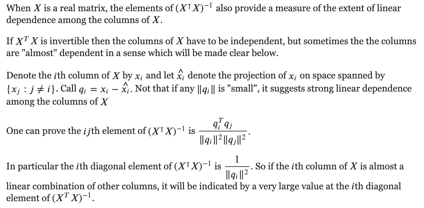
\[\widehat{\mathbb{Var}[\hat{\theta}]} = \widehat{\sigma^2} (X^\intercal X)^{-1} = \frac{(y - X \hat{\theta})^\intercal (y - X \hat{\theta})}{n - p} (X^\intercal X)^{-1}\]One result that remains to be confirmed is the following [9]:

References
[1] (1997) The problem of multicollinearity. In: Understanding Regression Analysis. Springer, Boston, MA
[2] Standard Errors in OLS. (n.d.). Home. https://lukesonnet.com/teaching/inference/200d_standard_errors.pdf
[3] Michael Hochster’s answer to why is multicollinearity bad in Layman’s terms? In feature selection for a regression model (intended for use in prediction), why is it a bad thing to have multicollinearity, or highly correlated independent variables? (n.d.). Quora - A place to share knowledge and better understand the world. https://www.quora.com/Why-is-multicollinearity-bad-in-laymans-terms-In-feature-selection-for-a-regression-model-intended-for-use-in-prediction-why-is-it-a-bad-thing-to-have-multicollinearity-or-highly-correlated-independent-variables/answer/Michael-Hochster
[4] Multicollinearity and predictive performance. (n.d.). Cross Validated. https://stats.stackexchange.com/questions/361247/multicollinearity-and-predictive-performance
[5] Multicollinearity. (2005, February 9). Wikipedia, the free encyclopedia. Retrieved June 9, 2020, from https://en.wikipedia.org/wiki/Multicollinearity
[6] Condition number. (2001, October 29). Wikipedia, the free encyclopedia. Retrieved June 9, 2020, from https://en.wikipedia.org/wiki/Condition_number
[7] https://www.statsmodels.org/dev/examples/notebooks/generated/ols.html#Condition-number
[8] Why is RSS distributed CHI square times n-P? (n.d.). Cross Validated. https://stats.stackexchange.com/questions/20227/why-is-rss-distributed-chi-square-times-n-p
[9] The meaning behind $(X^TX)^{-1}$. (n.d.). Mathematics Stack Exchange. https://math.stackexchange.com/questions/2624986/the-meaning-behind-xtx-1/2625661#2625661
[10] Model selection: Regression models. (n.d.). https://campus.datacamp.com/courses/practicing-machine-learning-interview-questions-in-python/model-selection-and-evaluation-4?ex=9