Gaussian distribution
One-dimensional case:
\[\mathbb{P}_{\mu, \sigma}(x) = \frac{1}{\sqrt{2\pi \sigma^2}} \exp(-\frac{(x-\mu)^2}{2\sigma^2})\]$d$-dimensional case:
\[\mathbb{P}_{\mu, \Sigma}(x) = \frac{1}{\sqrt{(2\pi)^d \det \Sigma}} \exp(-\frac{1}{2}(x-\mu)^\intercal \Sigma^{-1} (x-\mu))\]68–95–99.7 rule
The 68–95–99.7 rule is a shorthand used to remember the percentage of values that lie within one, two and three standard deviations of the mean in a normal distribution.
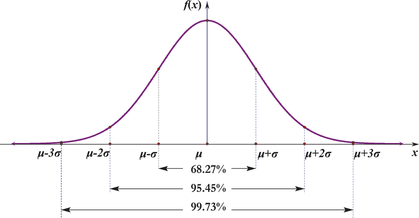
The three-sigma rule states that even for non-normally distributed variables, at least 88.8% of cases should fall within properly calculated three-sigma intervals. It follows from Chebyshev’s inequality. For unimodal distributions the probability of being within the interval is at least 95% by the Vysochanskij–Petunin inequality. There may be certain assumptions for a distribution that force this probability to be at least 98%.
Laplace distribution
One-dimensional case:
\[\mathbb{P}_{\mu, b}(x) = \frac{1}{2b} \exp(-\frac{|x - \mu|}{b})\]Mean: $\mu$
Variance: $2b^2$
Chi-squared distribution
$\chi^2$ distribution with $k$ degrees of freedom is denoted by $\chi_k^2$.
Mean: $k$
Variance: $2k$
Let $X_i \sim \mathcal{N}(0, 1)$, $X_i$’s are independent. $\overline{X} = \frac{1}{n} \sum_{i=1}^n X_i$.
\[\sum_{i=1}^n X_i^2 \sim \chi_n^2\] \[\sum_{i=1}^n (X_i - \overline{X})^2 \sim \chi_{n-1}^2\]Student’s t-distribution
Let $X_i \sim \mathcal{N}(\mu, \sigma^2)$, $X_i$’s are i.i.d.. $\overline{X} = \frac{1}{n} \sum_{i=1}^n X_i$, $S^2 = \frac{1}{n-1} \sum_{i=1}^n (X_i - \overline{X})^2$.
\[\frac{\overline{X} - \mu}{\frac{\sigma}{\sqrt{n}}} \sim \mathcal{N}(0, 1)\] \[t = \frac{\overline{X} - \mu}{\frac{S}{\sqrt{n}}}\]$t$ follows Student’s t-distribution with $n-1$ degrees of freedom.
Mean: $0$ for $\nu > 1$ degrees of freedom, otherwise undefined
F-distribution
F-distribution with parameters $d_1$ and $d_2$ is denoted by $F(d_1, d_2)$.
If $X_1 \sim \chi_{d_1}^2$ and $X_2 \sim \chi_{d_2}^2$ are independent, then
\[\frac{\frac{X_1}{d_1}}{\frac{X_2}{d_2}} \sim F(d_1, d_2)\]Mean: $\frac{d_2}{d_2 - 2}$ for $d_2 > 2$
Poisson distribution
Poisson distribution is a discrete probability distribution that expresses the probability of a given number of events occurring in a fixed interval of time or space if these events occur with a known constant mean rate and independently of the time since the last event.
A discrete random variable $X$ is said to have a Poisson distribution with parameter $\lambda > 0$, if $\forall k = 0, 1, 2, …,$
\[\mathbb{P}_{\lambda}(X = k) = \frac{\lambda^k e^{- \lambda} }{k!}\]Mean: $\lambda$
Variance: $\lambda$
Bernoulli distribution
\[\mathbb{P}_{p}(X=1) = 1 - \mathbb{P}_{p}(X=0) = p\]Mean: $p$
Variance: $p (1 - p)$
A Bernoulli trial (or binomial trial) is a random experiment with exactly two possible outcomes, “success” and “failure”, in which the probability of success is the same every time the experiment is conducted.
Binomial distribution 二项分布
\[\mathbb{P}_{n, p}(X = k) = {n \choose k} p^k (1 - p)^{n - k}\]Mean: $n p$
Variance: $n p (1 - p)$
Geometric distribution
The geometric distribution is either one of two discrete probability distributions:
- The probability distribution of the number $X$ of Bernoulli trials needed to get one success, supported on the set ${1, 2, 3, …}$.
- The probability distribution of the number $Y = X − 1$ of failures before the first success, supported on the set ${0, 1, 2, …}$.
Which of these is called “the” geometric distribution is a matter of convention and convenience. These two different geometric distributions should not be confused with each other.
The probability that the first occurrence of success requires $k$ independent trials, each with success probability $p$, i.e. the number of trials up to and including the first success or the probability that the kth trial (out of k trials) is the first success:
\[\mathbb{P}(X = k) = (1-p)^{k-1} p\]Mean: $\frac{1}{p}$
Variance: $\frac{1-p}{p^2}$
The number of failures $Y$ until the first success:
\[\mathbb{P}(Y = k) = (1-p)^{k} p\]Mean: $\frac{1 - p}{p}$
Variance: $\frac{1-p}{p^2}$
Laws
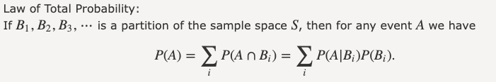
Law of total probability
Also known as:
- 全概率定理
Law of total expectation
Also known as:
- 全期望值定理
- law of iterated expectations
- tower rule
- Adam’s law
- smoothing theorem
- 双重期望值定理
- 重叠期望值定理
If $X$ is a random variable whose expected value $\mathbb{E}[X]$ is defined, and $Y$ is any random variable on the same probability space, then
\[\mathbb{E}[X] = \mathbb{E}[\mathbb{E}[X | Y]]\]i.e., the expected value of the conditional expectation of $X$ given $Y$ is the same as the expected value of $X$.
Law of total variance
Also known as:
- variance decomposition formula
- conditional variance formulas
- law of iterated variances
- Eve’s law
If $X$ and $Y$ are random variables on the same probability space, and the variance of $Y$ is finite, then
\[\mathbb{Var}[Y] = \mathbb{E}[\mathbb{Var}[Y | X]] + \mathbb{Var}[\mathbb{E}[Y | X]]\]For statisticians, the two terms are the “unexplained” and the “explained” components of the variance respectively. These two components are also the source of the term “Eve’s law”, from the initials EV VE for “expectation of variance” and “variance of expectation”.