By convention, $X \in \mathbb{R}^{n\times p}$ where $n$ denotes the number of samples, $p$ denotes the number of features. $x = (x_1, x_2, …, x_n)$.

PCA

Recall SVD, for any matrix $X\in \mathbb{R}^{n\times p}$,

\[X = U\Sigma V^\intercal\]

where $U\in \mathbb{R}^{n\times n}$, $V \in \mathbb{R}^{p\times p}$, $V^\intercal$ is the transpose of $V$. The columns of $U$ are called left singular vectors, the columns of $V$ are called right singular vectors. $U$ and $V$ are orthogonal matrices.

To compute PCA for $X\in \mathbb{R}^{n\times p}$,

For each column/feature of $X$, substract the mean. Optionally, one can also divide the standard deviation for each column, this seems to be recommended. Call the resulted matrix $\tilde{X}\in \mathbb{R}^{n\times p}$.
Compute SVD of $\tilde{X}$, one obtains $\tilde{X} = U\Sigma V^\intercal$. The columns of $V$ (right singular vectors) are called principal components. Equivalently, this is to compute eigendecomposition of $\tilde{X}^\intercal \tilde{X} \in \mathbb{R}^{p\times p}$, i.e. $\tilde{X}^\intercal \tilde{X} = P S P^{-1}$. $\tilde{X}^\intercal \tilde{X}$ is the empirical covariance matrix between features up to a normalization constant ($\frac{1}{n}$ or $\frac{1}{n - 1}$ if using Bessel’s correction). The right singular vectors of $\tilde{X}$ are the eigenvectors of $\tilde{X}^\intercal \tilde{X}$, that is, $\tilde{X}^\intercal \tilde{X} = V\Sigma U^\intercal U\Sigma V^\intercal = V\Sigma^2 V^\intercal = V S V^\intercal = V S V^{-1} = P S P^{-1}$. By convention, the singular values are sorted in descending order, singular vectors are sorted accordingly.
$X^* = \tilde{X} V = U\Sigma \in \mathbb{R}^{n\times p}$ is the transformed version of $X$ by PCA. So far, one uses a new orthogonal basis to represent data $X$. If one seeks for dimensionality reduction, one only keeps the $k$ principal components which correspond to the $k$ largest singular values. That is, $V_k \in \mathbb{R}^{p\times k}$, $X_k^* = \tilde{X} V_k \in \mathbb{R}^{n\times k}$.
For unseen test data $Z\in \mathbb{R}^{m\times p}$, normalize it with the statistics (means, standard deviations) of training set and then do the matrix multiplication $Z_k^* = \tilde{Z}V_k \in \mathbb{R}^{m\times k}$. One should neither use statistics of test set to normalize nor compute the statistics using the whole dataset (training + test). The principal components are of course those computed from training set.

For symmetric positive semidefinite matrices such as the empirical covariance matrix $\tilde{X}^\intercal \tilde{X}$, the SVD and the eigendecomposition give the same result, they are mathematically equivalent. Numerically, this might not be the case because they can use different algorithms. Andrew Ng says that SVD is numerically more stable than eigendecomposition. An attempt to explain this is that the SVD implementation seems to be using a divide-and-conquer approach (LAPACK), while the eigendecomposition uses a plain QR algorithm. This explanation remains to be confirmed.

MLE & MAP

Maximum likelihood estimation (MLE):

\[\begin{equation} \begin{split} \hat{\theta}_{\text{MLE}} &= \underset{\theta}{\operatorname{argmax}} \log \mathbb{P}_\theta (x) = \underset{\theta}{\operatorname{argmax}} \log \mathbb{P} (x | \theta) \\ &= \underset{\theta}{\operatorname{argmax}} \sum_i \log \mathbb{P} (x_i | \theta) \end{split} \end{equation}\]

Maximum a posteriori (MAP):

\[\begin{equation} \begin{split} \hat{\theta}_{\text{MAP}} &= \underset{\theta}{\operatorname{argmax}} \log \mathbb{P} (\theta | x) \\ &= \underset{\theta}{\operatorname{argmax}} \log \frac{\mathbb{P} (x | \theta) \mathbb{P}(\theta)}{\mathbb{P}(x)} \\ &= \underset{\theta}{\operatorname{argmax}} \log \mathbb{P} (x | \theta) \mathbb{P}(\theta) \\ &= \underset{\theta}{\operatorname{argmax}} \sum_i \log \mathbb{P} (x_i | \theta) + \log \mathbb{P}(\theta) \end{split} \end{equation}\]

If the prior $\mathbb{P}(\theta)$ is uniform, then MAP reduces to MLE. MAP can be seen as MLE augmented with a regularization term. If the prior is assumed to be centered Gaussian distribution $\mathcal{N}(\boldsymbol{0}, \frac{1}{\lambda} I)$, then this is $L2$ regularization, that is, $-\log \mathbb{P}(\theta) = \frac{\lambda}{2}\vert\vert\theta\vert\vert_2^2$. If the prior is assumed to be centered Laplace distribution, then this is $L1$ regularization.

Linear regression

There are 4 principal assumptions which justify the use of linear regression models for purposes of inference or prediction [1]:

linearity and additivity of the relationship between dependent variables (target variables) and independent variables (features)
- the expected value of dependent variable is a straight-line function of each independent variable, holding the others fixed
- the slope of that line does not depend on the values of the other variables
- the effects of different independent variables on the expected value of the dependent variable are additive
statistical independence of the errors (in particular, no correlation between consecutive errors in the case of time series data)
homoscedasticity (constant variance, 同方差性) of the errors
- versus time (in the case of time series data)
- versus the predictions
- versus any independent variable
normality of the error distribution

If any of these assumptions is violated, then the forecasts, confidence intervals, and scientific insights yielded by a regression model may be (at best) inefficient or (at worst) seriously biased or misleading.

\[y = X\theta^* + \epsilon\]

Ordinary least squares (OLS)

\[\hat{\theta} \in \underset{\theta}{\operatorname{argmin}} \frac{1}{2} \vert\vert X\theta - y \vert\vert_2^2\]

Method 1:

\[\nabla_\theta \frac{1}{2} \vert\vert X\theta - y \vert\vert_2^2 = X^\intercal (X\theta - y) = 0\]

Method 2:

\[f(\theta) = \frac{1}{2} \vert\vert X\theta - y \vert\vert_2^2 = \frac{1}{2} \theta^\intercal X^\intercal X\theta - \langle \theta, X^\intercal y \rangle + \frac{1}{2} \vert\vert y \vert\vert^2\] \[f(\theta + h) = f(\theta) + \langle h, X^\intercal X\theta - X^\intercal y \rangle + \frac{1}{2} h^\intercal X^\intercal Xh\]

According to the first-order Taylor series approximation $f(\theta + h) = f(\theta) + \langle h, \nabla f(\theta) \rangle + o(h)$, $\nabla f(\theta) = X^\intercal X\theta - X^\intercal y $.

Method 3:

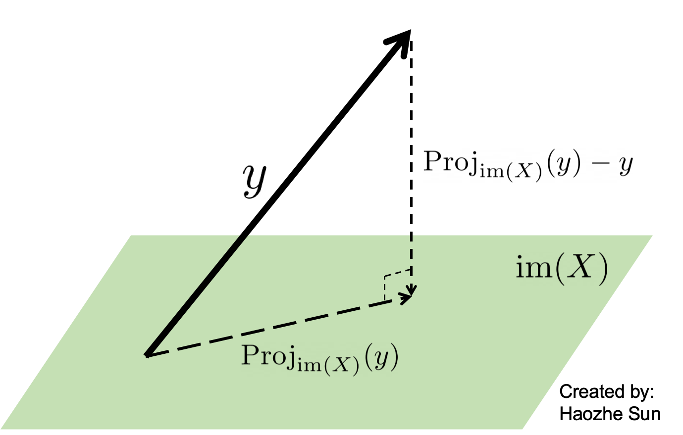
One aims to find $\theta$ such that $y = X\theta$. However, as $y \notin \text{im}(X)$, where $\text{im}(X)$ denotes the column space of $X$, one instead solves $\text{Proj}_{\text{im}(X)}(y) = X\theta$.

\[\begin{equation} \begin{split} & X\theta - y = \text{Proj}_{\text{im}(X)}(y) - y \\ & \text{Proj}_{\text{im}(X)}(y) - y \in \text{im}(X)^\perp \end{split} \end{equation}\] \[\Downarrow\] \[X\theta - y \in \text{im}(X)^\perp\]

As $\text{im}(X)^\perp = \ker(X^\intercal)$, $X^\intercal (X\theta - y) = 0$.

Theorem: If the columns of $X$ are linearly independent, then $X^\intercal X$ is invertible and $X^\intercal X \theta = X^\intercal y$ has a unique solution $\hat{\theta} = (X^\intercal X)^{-1}X^\intercal y$.

Proof: Let $\theta \in \ker(X^\intercal X)$, that is, $X^\intercal X \theta = 0$. Then,

\[\begin{equation}\begin{split} & \theta^\intercal X^\intercal X\theta = \vert\vert X\theta \vert\vert^2 = 0 \\ \Rightarrow & X\theta = \theta_1 \text{col}_1(X) + \theta_2 \text{col}_2(X) + ... = 0 \end{split}\end{equation}\]

As the columns of $X$ are linearly independent, $\theta = 0$, $\ker(X^\intercal X) = {0}$.

OLS estimator is the best linear unbiased estimator. Ridge regression has higher bias and lower variance than OLS.

Ridge regression

\[\hat{\theta} \in \underset{\theta}{\operatorname{argmin}} \frac{1}{2} \vert\vert X\theta - y \vert\vert_2^2 + \frac{\lambda}{2} \vert\vert \theta \vert\vert_2^2\] \[\nabla_\theta \frac{1}{2} \vert\vert X\theta - y \vert\vert_2^2 + \frac{\lambda}{2} \vert\vert \theta \vert\vert_2^2 = 0 \Rightarrow \hat{\theta} = (X^\intercal X + \lambda I)^{-1}X^\intercal y\]

Coefficient of determination

The most general definition of the coefficient of determination is

\[R^2 = 1 - \frac{\text{residual sum of squares}}{\text{total sum of squares}} = 1 - \frac{\text{残差平方和}}{\text{总平方和}} = 1 - \frac{\sum_i (y_i - f_i)^2}{\sum_i (y_i - \overline{y})^2} = 1 - \frac{\frac{1}{n} \sum_i (y_i - f_i)^2}{\frac{1}{n} \sum_i (y_i - \overline{y})^2} = 1 - \frac{\text{mean squared error}}{\text{variance}}\]

where

\[\overline{y} = \frac{1}{n} \sum_i^n y_i\]

$y_1$, $y_2$, …, $y_n$ denotes the $n$ target variables, $f_1$, $f_2$, …, $f_n$ denotes the $n$ predicted values by our model.

Values of $R^2$ outside the range $0$ to $1$ can occur when the model fits the data worse than a horizontal hyperplane.

$R^2$ (R squared) can be interpreted as the proportion of the variance in the target variable (label) that is predictable from the features. It is $1$ minus the “normalized” mean squared error (normalized by the variance of the target/label variables).

Logistic regression

Suppose $w, x \in \mathbb{R}^{p+1}$, the bias term is included. Capital letters indicate random variables.

\[\mathbb{P}(Y=1 | x) = \frac{1}{1 + \exp{(-w^\intercal x)} }\] \[w^\intercal x = \log \frac{\mathbb{P}(Y=1 | x)}{1 - \mathbb{P}(Y=1 | x)} = \text{logit}(\;\mathbb{P}(Y=1 | x)\;)\]

The function $\text{logit}(\cdot)$ is called log-odds or logit function.

Use MLE to estimate the parameter $w$.

If $y\in {0, 1}$,

\[\begin{equation} \begin{split} \underset{w}{\mathrm{argmax}}\; L(w) &= \underset{w}{\mathrm{argmax}}\; \log \prod_{i} \mathbb{P}(Y=1 | x_i)^{y_i} (1 - \mathbb{P}(Y=1 | x_i)\;)^{1-y_i} \\ &= \underset{w}{\mathrm{argmax}}\; \sum_i y_i \log \mathbb{P}(Y=1 | x_i) + (1-y_i) \log(1 - \mathbb{P}(Y=1 | x_i) \;) \\ &= \underset{w}{\mathrm{argmax}}\; \sum_i y_i \log \frac{\mathbb{P}(Y=1 | x_i)}{1 - \mathbb{P}(Y=1 | x_i)} + \log(1 - \mathbb{P}(Y=1 | x_i) \;) \\ &= \underset{w}{\mathrm{argmin}}\; \sum_i \log(1 + \exp(w^\intercal x)\;) - y_i w^\intercal x_i \end{split} \end{equation}\] \[\begin{equation} \begin{split} \nabla_w L(w) &= \sum_i \frac{1}{1 + \exp(- w^\intercal x_i)\;} x_i - y_i x_i \\ &= \sum_i (\frac{1}{1 + \exp(- w^\intercal x_i)\;} - y_i) x_i \end{split} \end{equation}\]

If $y\in {-1, 1}$,

\[\begin{equation} \begin{split} \underset{w}{\mathrm{argmax}}\; L(w) &= \underset{w}{\mathrm{argmax}}\; \log \prod_i \mathbb{P}(Y=y_i | x_i) \\ &= \underset{w}{\mathrm{argmax}}\; \log \prod_i \frac{1}{1 + \exp(-y_i w^\intercal x_i)} \\ &= \underset{w}{\mathrm{argmin}}\; \sum_i \log(1 + \exp(-y_i w^\intercal x_i)\;) \end{split} \end{equation}\] \[\begin{equation} \begin{split} \nabla_w L(w) &= \sum_i \frac{- y_i}{1 + \exp(y_i w^\intercal x_i)} x_i \end{split} \end{equation}\]

SVM

Suppose $w, x \in \mathbb{R}^{p}$, the bias term is not included. $y\in {-1, 1}$.

If the training data is linearly separable, hard-margin SVM.

The primal form:

\[\begin{equation}\begin{split} &\min_{w,b} \quad \quad \quad \frac{1}{2} ||w||^2 \\ &\text{s.t.} \quad 1 - y_i (w^\intercal x_i + b) \leqslant 0, \forall i \end{split}\end{equation}\]

The dual form:

\[\begin{equation}\begin{split} &\min_{\alpha} \quad \quad \quad \frac{1}{2} \sum_i \sum_j \alpha_i \alpha_j y_i y_j x_i^\intercal x_j - \sum_i \alpha_i \\ &\text{s.t.} \quad \alpha_i \geqslant 0, \forall i \\ & \quad \quad \sum_i \alpha_i y_i = 0, \forall i \end{split}\end{equation}\]

There exists $j$ such that $\alpha_j^* > 0$,

\[w^* = \sum_i \alpha_i^* y_i x_i\] \[b^* = y_j - \sum_i \alpha_i^* y_i x_i^\intercal x_j\]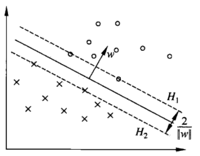

If the training data is not linearly separable, soft-margin SVM.

The primal form:

\[\begin{equation}\begin{split} &\min_{w,b,\xi} \quad \quad \quad \frac{1}{2} ||w||^2 + C \sum_i \xi_i \\ &\text{s.t.} \quad 1 - y_i (w^\intercal x_i + b) \leqslant \xi_i, \forall i \\ & \quad \quad \xi_i \geqslant 0, \forall i \end{split}\end{equation}\]

The dual form:

\[\begin{equation}\begin{split} &\min_{\alpha} \quad \quad \quad \frac{1}{2} \sum_i \sum_j \alpha_i \alpha_j y_i y_j x_i^\intercal x_j - \sum_i \alpha_i \\ &\text{s.t.} \quad 0 \leqslant \alpha_i \leqslant C, \forall i \\ & \quad \quad \sum_i \alpha_i y_i = 0, \forall i \end{split}\end{equation}\]

There exists $j$ such that $0 < \alpha_j^* < C$,

\[w^* = \sum_i \alpha_i^* y_i x_i\] \[b^* = y_j - \sum_i \alpha_i^* y_i x_i^\intercal x_j\]

Soft-margin SVM can be written as the hinge loss with regularization term.

\[\begin{equation}\begin{split} \min_{w,b} \sum_i \max(1-y_i (w^\intercal x_i + b), 0) + \lambda ||w||^2 \end{split}\end{equation}\]

Lagrangian function

\[\begin{equation}\begin{split} &\min_{x} \quad \quad \quad f(x) \\ &\text{s.t.} \quad g_i(x) \leqslant 0, \forall i \\ & \quad \quad h_j(x) = 0, \forall j \end{split}\end{equation}\]

The Lagrangian function is formed as follows:

\[\mathcal{L}(x,\mu,\lambda) = f(x) + \mu^\intercal g(x) + \lambda^\intercal h(x)\]

KKT conditions

First order primal optimality

\[\nabla_x \mathcal{L}(x, \mu, \lambda) = 0\]

Primal feasibility

\[g_i (x^*) \leqslant 0, \forall i\] \[h_j(x^*) = 0, \forall j\]

Dual feasibility

\[\mu_i \geqslant 0, \forall i\]

Complementary slackness

\[\mu_i g_i (x^*) = 0, \forall i\]

Tf–idf

One way to define tf–idf (term frequency–inverse document frequency) is the following:

\[w_{i,j} = \text{t}_{i,j} \log \frac{D}{\text{d}_i}\]

where $w_{i,j}$ is the tf-idf weight for token $i$ in document $j$, $t_{i,j}$ is the number of occurences of token $i$ in document $j$, $d_{i}$ is the number of documents that contain token $i$, $D$ is the total number of documents.

However other ways of defining the term frequency and the document frequency exist, for example, normalization, smoothing, etc.

Convolutional neural networks

To compute the output width (resp. height) of a 2D convolutional layer, suppose the kernel size $F$, the stride $S$, the amount of zero padding $P$, the input width (resp. height) $I$, the output width (resp. height) $O$:

\[O = \frac{(I - F + 2P)}{S} + 1\]

To compute the output width (resp. height) of a 2D pooling layer, suppose the kernel size $F$, the stride $S$, the input width (resp. height) $I$, the output width (resp. height) $O$:

\[O = \frac{I - F}{S} + 1\]

A 2D convolutional layer with $F=3, P=1, S=1$ will not change the width (resp. height): $O=I$, a 2D pooling layer with $F=2, S=2$ will produce $O = \frac{I}{2}$ (without remainder).

Reinforcement learning (RL)

In applications where there is a natural notion of final time step, an episode is a (sub)sequence of agent–environment interactions, such as plays of a game, trips through a maze, or any sort of repeated interactions. Each episode ends in a special state called the terminal state, followed by a reset to a standard starting state or to a sample from a standard distribution of starting states. Tasks with episodes of this kind are called episodic tasks. On the other hand, in many cases the agent–environment interaction does not break naturally into identifiable episodes, but goes on continually without limit. We call these continuing tasks.

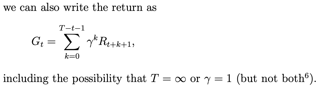
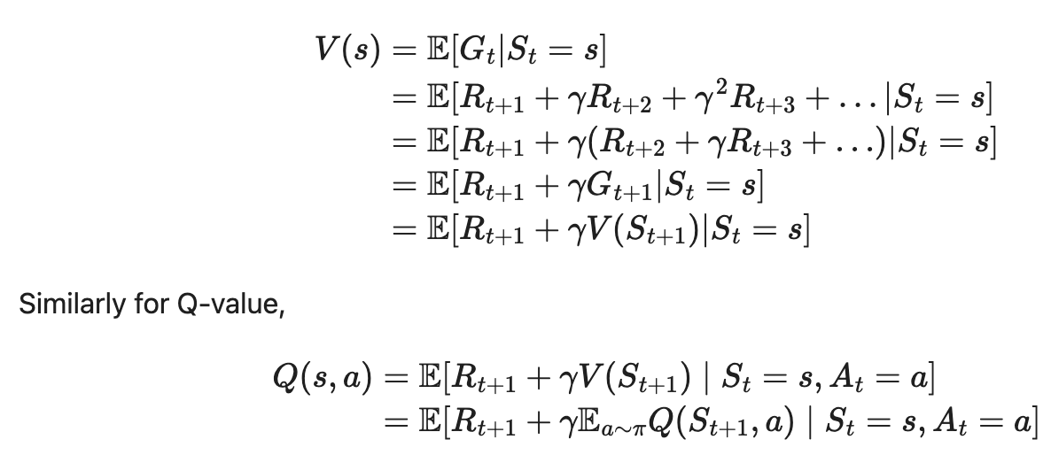
General definition of return:

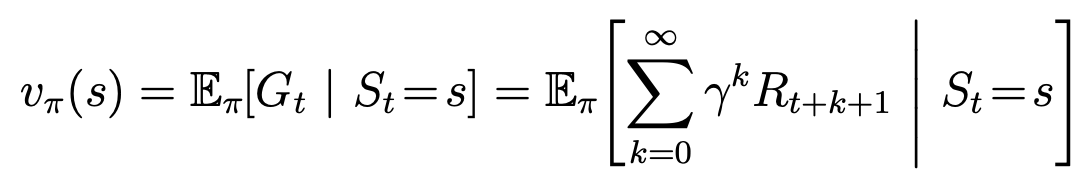
Definition of state value function for policy $\pi$:

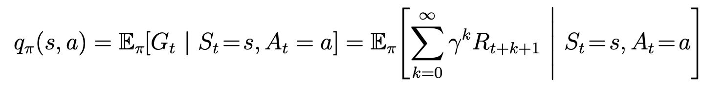
Definition of action value function for policy $\pi$:

Bellman equations refer to a set of equations that decompose the value function into the immediate reward plus the discounted future values.

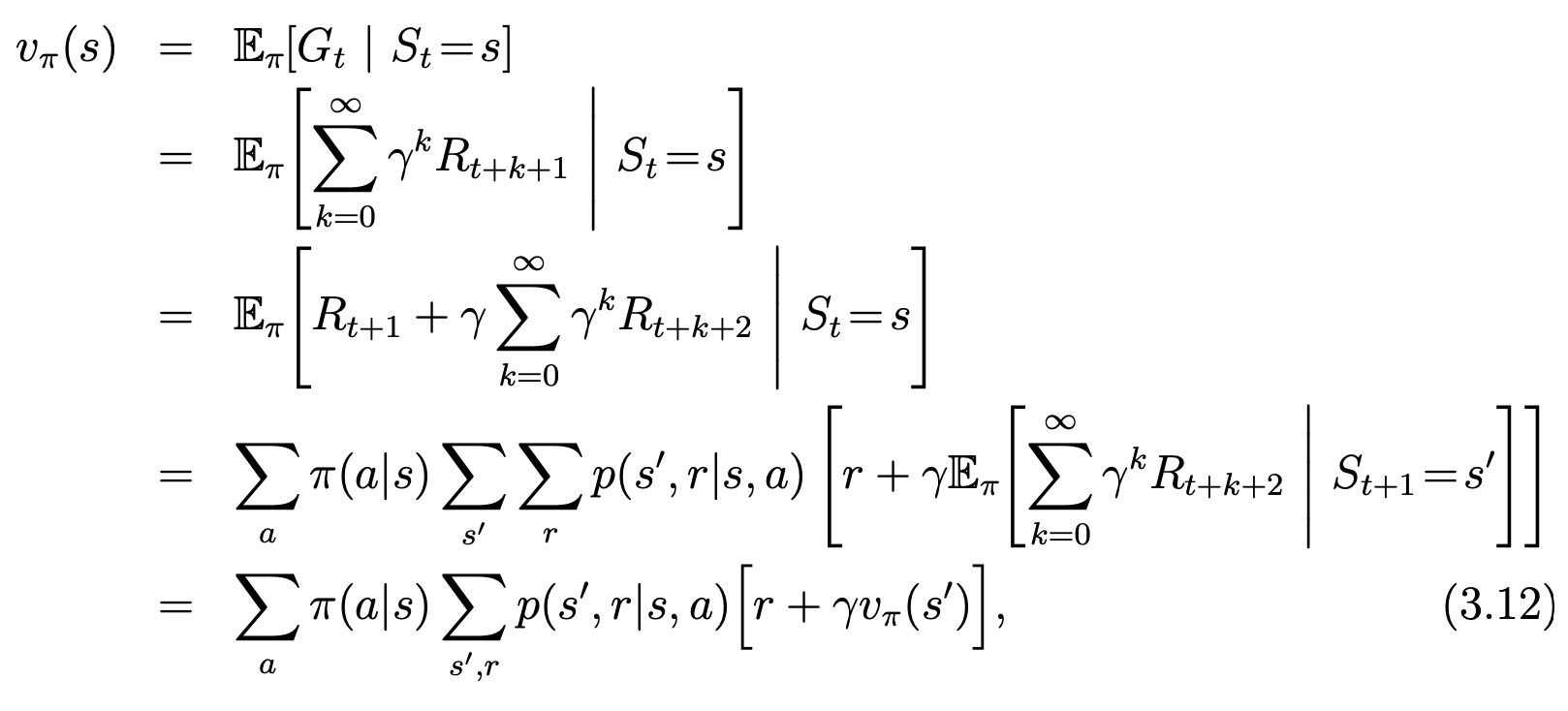
Bellman equation for state value functions (relationship between the value of a state and the values of its successor states):

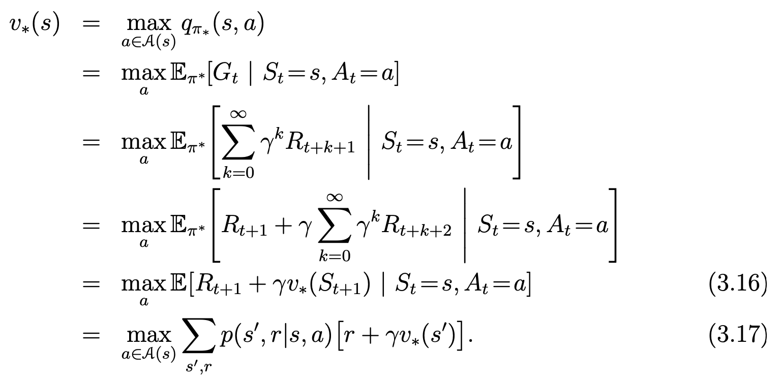
Bellman optimality equation for state value functions:

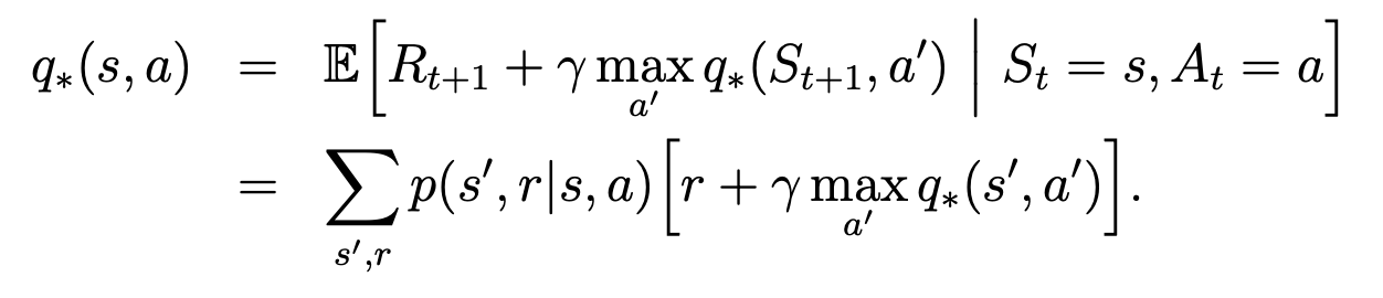
Bellman optimality equation for action value functions:

Bellman equations according to Lilian Weng:

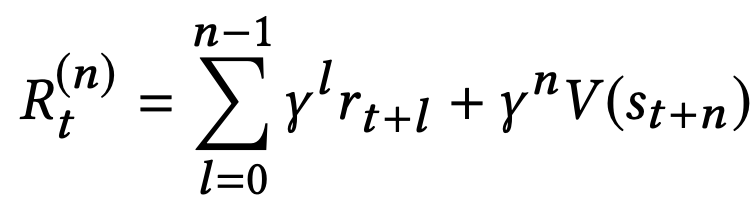
The n-step return can be computed by truncating the sum of returns after n steps, and approximating the return from the remaining steps using a value function V(s):

1-step return:

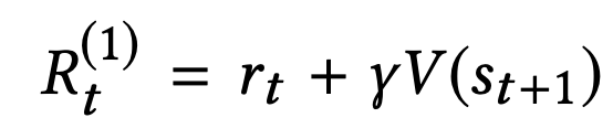
In n-step returns, $n$ acts as a trade-off between bias and variance for the value estimator. While $R_t^{(∞)}$ provides an unbiased but high variance estimator, $R_t^{(1)}$ provides a biased but low variance estimator.

Another method to trade off between the bias and variance of the estimator is to use a λ-return, calculated as an exponentially-weighted average of n-step returns with decay parameter λ:

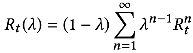
λ = 0 reduces to the single-step return $R_t^{(1)}$, and λ = 1 recovers the Monte-Carlo return $R_t^{(∞)}$. Intermediate values of $\lambda \in (0, 1)$ produces interpolants that can be used to balance the bias and variance of the value estimator.

When the model is fully known, following Bellman equations, we can use Dynamic Programming (DP) to iteratively evaluate value functions and improve policy.

Policy Evaluation is to compute the state-value
Based on the value functions, Policy Improvement generates a better policy by acting greedily.
The Generalized Policy Iteration (GPI) algorithm refers to an iterative procedure to improve the policy when combining policy evaluation and improvement.

Monte-Carlo (MC) methods need to learn from complete episodes to compute returns and all the episodes must eventually terminate.

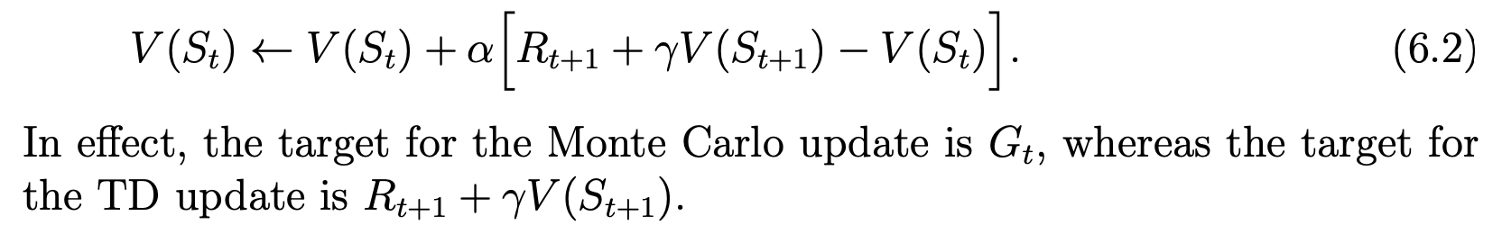
Similar to Monte-Carlo methods, Temporal-Difference (TD) Learning is model-free. However, TD learning can learn from incomplete episodes. TD learning methods update targets with regard to existing estimates rather than exclusively relying on actual rewards and complete returns as in MC methods. This approach is known as bootstrapping. Temporal difference (TD) methods learn a guess from a guess, they bootstrap.

TD(0), which is the simplest TD method:

Methods in which the temporal difference extends over $n$ steps are called n-step TD methods. We are free to pick any $n$ in TD learning as we like. Now the question becomes what is the best $n$? A common yet smart solution is to apply a weighted sum of all possible n-step TD targets rather than to pick a single best $n$. The weights decay by a factor λ with $n$, $\lambda^{n-1}$. the intuition is similar to why we want to discount future rewards when computing the return: the more future we look into the less confident we would be. This weighted sum of many n-step returns is called λ-return.

TD(λ):

Updating the value function using the temporal difference computed with the λ-return results in the TD(λ) algorithm.
TD learning that adopts λ-return for value updating is labeled as TD(λ).
The TD(λ) algorithm can be understood as one particular way of averaging n-step TD targets. This average contains all the n-step TD targets, each weighted proportional to $\lambda^{n-1}$, and normalized by a factor of (1 − λ) to ensure that the weights sum to 1.

In the TD(λ) algorithm, the λ refers to the use of an eligibility trace. There are two ways to view eligibility traces:

The more theoretical view (forward view), is that they are a bridge from TD to Monte Carlo methods. When TD methods are augmented with eligibility traces, they pro- duce a family of methods spanning a spectrum that has Monte Carlo methods at one end and one-step TD methods at the other. In between are intermediate methods that are often better than either extreme method. The forward view is most useful for understanding what is computed by methods using eligibility traces.
The other way (backward view) to view eligibility traces is more mechanistic. From this perspective, an eligibility trace is a temporary record of the occurrence of an event, such as the visiting of a state or the taking of an action. The trace marks the memory parameters associated with the event as eligible for un- dergoing learning changes. When a TD error occurs, only the eligible states or actions are assigned credit or blame for the error. Thus, eligibility traces help bridge the gap between events and training information. The backward view is more appropriate for developing intuition about the algorithms themselves.

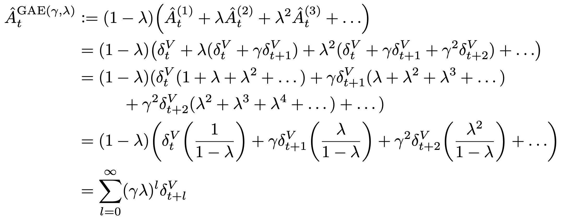
The Generalized Advantage Estimator GAE(γ, λ) is defined as the exponentially-weighted average of the k-step advantage estimators (discounted by $\lambda$). It is also the infinite sum of future TD errors, exponentially discounted by $(\gamma \lambda)$.

Each k-step advantage estimator is defined to be the exponentially discounted sum of the next k TD errors (discounted by $\gamma$).
Each k-step advantage estimator is also a k-step estimate of the returns, minus a baseline term $V(s_t)$ (the value of the current state).

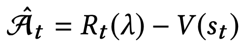
Estimating the advantage with the λ-return yields the Generalized Advantage Estimator (GAE). TD(λ) is an estimator of the value function, whereas GAE is estimating the advantage function.

Generalized Advantage Estimator GAE(γ, λ):

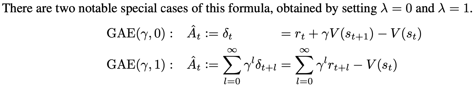
In GAE, both $\gamma$ and $\lambda$ contribute to the bias-variance tradeoff when using an approximate value function. However, they serve different purposes and work best with different ranges of values.

$\gamma$ most importantly determines the scale of the value function $V^{\pi, \gamma}$, which does not depend on $\lambda$.
Taking $\gamma < 1$ introduces bias into the policy gradient estimate, regardless of the value function’s accuracy.
Taking $\lambda < 1$ introduces bias only when the value function is inaccurate.
Empirically, we find that the best value of $\lambda$ is much lower than the best value of $\gamma$, likely because $\lambda$ introduces far less bias than $\gamma$ for a reasonably accurate value function.
In the original GAE paper which mainly considers simulated robotic locomotion tasks, $\lambda$ in the range [0.9, 0.99] usually results in the best performance.

TD control:

SARSA: On-Policy TD control. “SARSA” refers to the procedure of updaing Q-value by following a sequence of state, action, reward, state, action, etc. In each step of SARSA, we need to choose the next action according to the current policy.
Q-Learning: Off-policy TD control. The key difference from SARSA is that Q-learning does not follow the current policy to pick the second action.

References

[1] Testing the assumptions of linear regression. (n.d.). people.duke.edu. https://people.duke.edu/~rnau/testing.htm

[2] Sutton, Richard S., and Andrew G. Barto. Reinforcement Learning: An Introduction. Second. The MIT Press, 2018. http://incompleteideas.net/book/the-book-2nd.html.

[3] Schulman, John, Philipp Moritz, Sergey Levine, Michael Jordan, and Pieter Abbeel. “High-Dimensional Continuous Control Using Generalized Advantage Estimation.” arXiv E-Prints, June 2015, arXiv:1506.02438.

[4] Weng, Lilian. A (Long) Peek into Reinforcement Learning. 2018. https://lilianweng.github.io/posts/2018-02-19-rl-overview/

[5] Peng, Xue Bin, Pieter Abbeel, Sergey Levine, and Michiel van de Panne. “DeepMimic: Example-Guided Deep Reinforcement Learning of Physics-Based Character Skills.” arXiv, July 27, 2018. http://arxiv.org/abs/1804.02717.